A new (3+1) dimensional Hirota bilinear equation: Painlavé integrability, Lie symmetry analysis, and conservation laws

Abstract

This study's subject is a (3 + 1) dimensional new Hirota bilinear (NHB) equation that appears in the theory of shallow water waves. We investigate how particular dispersive waves behave in an NHB equation. In this regard, we first test the Painlavé integrability using the WTC-Kruskal method and second perform Lie point symmetry analysis on NHB. The algorithm outputs the Lie algebra, the symmetry reductions, and group invariant solutions. Using Lie point symmetries, NHB transforms into an ordinary differential equation. The integration architectures to solve this equation are the Bernoulli sub-ODE, 1/ G${}^{\prime }$, and modified Kudryashov methods. We plot their graphs and observe how the solutions behaved in understanding the physical phenomenon. Additionally, we discuss the model utilizing nonlinear self-adjointness and Ibragimov's approach to generate conservation laws for each Lie symmetry generator.

Keywords:

• Painlevé analysis
• Lie symmetry
• group-invariant solutions
• conservation laws

1. Introduction

Materials science, ocean engineering, biology, solid state physics, chemistry, chemical physics, optical fibers, chemical kinetics, deep water waves, oceanography, signal processing, and all other nonlinear disciplines use nonlinear evolution equations (NLEE). A NLEE is a partial differential equation that explains how a physical system changes over time and under a set of given initial conditions. It affects physical processes such as system identification that appear beyond several scientific disciplines.

Energy is moved from one location to another through waves. The ocean's water level will rise and fall in intricate and unpredictable motions while transferring energy from a region of disturbance due to forces that include gravity and wind, as well as other factors like gravity or movement of the ocean floor. An ocean wave is the term used to describe this energy transfer via the ocean's surface water [1]. The dynamic waves that characterize marine environments, examine sea movement, and display tropical tidal waves are the shallow water waves. These waves form as a result of wind activity on the sea and show long wavelength wonders where level length is more important than liquid depth. Sea foot influences these waves as they proliferate, aggravating the water's orbital movement. It might then result in unimaginable destruction to the coastal ecology, among other things [2]. If the contact of the wave with the sea or ocean floor is having an impact on the waves at the surface, ocean waves are regarded as shallow water waves [1].

As utilized in physical sciences, the exact solution for the most part alludes to an arrangement that captures the complete nature of a problem as contradicted to one that is approximate and perturbation solutions.

Setting up exact analytical solutions of NLEEs is imperative since it better portrays the physical phenomena. Exact analytical solutions are extremely beneficial for testing numerical algorithms used for the considered equation.

Group-invariant solutions, which is a special class of exact solutions, are the solution forms obtained by the Lie symmetry groups approach and remaining invariant through various geometric transformations of the considered model.

Conservation laws, which were closely related through Lie symmetry groups at the beginning of the twentieth century and which are quite well known in physical sciences, are the basic building blocks in the linearization of the equation, the use of numerical schemes and stability analysis, as well as the inference of the basic conservation laws of the model under consideration.

To obtain the exact solutions of NLEEs, various techniques, including Hirota bilinear theory [3], Darboux transformation [4], Painlavé analysis [5], Lie symmetry analysis [6], Bernoulli sub-ODE method [7], $\left({\displaystyle \frac{G}{G^{\prime }}}\right)$-expansion [8], the modified (G ${}^{\prime }$ /G)-expansion method [9], etc. were suggested in the literature. Some of the methods have even been used for fractional differential equations [10, 11].

A self-reinforcing single wave within a wave container is referred to as a soliton if it continually maintains its form while moving at a fixed pace. Solitons are constructed by arranging a variety of dispersive NLEEs to represent physical structures [12].

The (1+1)-dimensional Korteweg–de Vries (KdV) equation (1) $u_t+6u{u}_x+u_{xxx}=0$(1) is a NLEE which is conventionally employed to model the behaviour of waves in shallow water.

Another NLEE that expresses the development of nonlinear, long waves with small amplitudes and gradual reliance on the transverse coordinate is the Kadomtsev–Petviashvili (KP) equation, which has two spatial and one temporal variables. The KP equation has two unique forms and may be expressed as follows in the normalized form: (2) $(u_t+6u{u}_x+u_{xxx}{)}_x+3{\vartheta }^2{u}_{yy}=0,$(2) where $u=u(x,y,t)$ may be a scalar function, x and y are separately the longitudinal and transverse spatial coordinates, and ${\vartheta }^2=\pm 1$. The KPII equation is known under the case $\vartheta =1$, and miniatures, for example, water waves with low surface pressure. The KPI equation, which may be used to demonstrate pulses in thin films with high surface pressure, is known under the case $\vartheta =i$.

One of the such NLEEs (extended and high-dimensional version of the KdV equation) mentioned above lines is the following $(3+1)$-dimensional new Hirota bilinear (NHB) equation [13–15] (3) $u_{yt}-u_{xxxy}-3(u_x{u}_y{)}_x-3u_{xx}+3u_{zz}=0.$(3) Equation (3(3) $u_{yt}-u_{xxxy}-3(u_x{u}_y{)}_x-3u_{xx}+3u_{zz}=0.$(3) ) is transformed into the KdV equation (4) $W_P+6W{W}_R+W_{RRR}=0$(4) by using the transformations t = −P, x = −R, y = Q, z = Q and $u_x=W$.

Equation (4(4) $W_P+6W{W}_R+W_{RRR}=0$(4) ) has N-soliton solutions via Hirota perturbation theory and is totally integrable. The literature on Equation (3(3) $u_{yt}-u_{xxxy}-3(u_x{u}_y{)}_x-3u_{xx}+3u_{zz}=0.$(3) ) reveals a number of ongoing studies. Equation (3(3) $u_{yt}-u_{xxxy}-3(u_x{u}_y{)}_x-3u_{xx}+3u_{zz}=0.$(3) ) was solved using the linear superposition approach in [13], and two different resonant multiple wave solutions were discovered. Also, lump solutions to two different dimensional reductions with z = y and z = t in [14]. Bilinear Bäcklund transformation is shown in [16]. The N-solitary waves are further obtained in [17] depending on the resulting bilinear form by applying Hirota's bilinear theory. In [18], a periodic type II, rogue, bright, and dark wave evolution of Equation (3(3) $u_{yt}-u_{xxxy}-3(u_x{u}_y{)}_x-3u_{xx}+3u_{zz}=0.$(3) ) with physical properties was developed.

The primary objective of this study is to carry out invariance analysis of the (3+1) dimensional NHB equation model, which emerged in shallow-water wave theory, through the technique of Lie-symmetry groups. In this way, variable changes corresponding to various geometric transformations and the formation of new reduced versions of the model and new exact (group invariant) solution forms will be investigated. However, the formation of local conservation vectors, which we cannot observe for this model, will also be demonstrated with the help of Lie symmetry groups and a coupled version of Noether's theorem developed by Ibragimov [19].

This study consists of the following sections. In Section 2, we investigate the Painlavé integrability of Equation (3(3) $u_{yt}-u_{xxxy}-3(u_x{u}_y{)}_x-3u_{xx}+3u_{zz}=0.$(3) ) using the WTC-Kruskal algorithm [20–24]. In Sections 3 and 4, using Lie algebra [25–30], we take into consideration the (3+1) dimensional Hirota equation. We investigate the Lie infinitesimals for Equation (3(3) $u_{yt}-u_{xxxy}-3(u_x{u}_y{)}_x-3u_{xx}+3u_{zz}=0.$(3) ) using the fourth prolongation. We reduce Equation (3(3) $u_{yt}-u_{xxxy}-3(u_x{u}_y{)}_x-3u_{xx}+3u_{zz}=0.$(3) ) to ODEs using some generators and their combinations. In Section 5 we have to reach at the solutions of the ODE's and, consequently, various solutions of Equation (3(3) $u_{yt}-u_{xxxy}-3(u_x{u}_y{)}_x-3u_{xx}+3u_{zz}=0.$(3) ) using the Bernoulli Sub-Ode, ${\displaystyle \frac{1}{G^{\mathrm{\prime }}}}$ and modified Kudryashov approaches mentioned in [7]. In Section 6, as stated in [31], we study and determine the quasi self-adjointness of Equation (3(3) $u_{yt}-u_{xxxy}-3(u_x{u}_y{)}_x-3u_{xx}+3u_{zz}=0.$(3) ). Again in this section, we calculate the conservation vectors using Ibragimov's method [19, 31]. In the Conclusion section we obtain 3D graphs of the solutions and analyse their behaviour over time, in order to better understand the physical phenomenon behind the model. In the last, we provide an overview of the study and conclusions.

2. Painlavé analysis

According to [20], consider an NLEE, for example one dependent variable with respect to independent variables x, y, z, and t, (5) $P(u,u_x,u_y,u_z,u_t,\dots )=0,$(5) where $u(x,y,z,t)$ is the dependent variable, P is a polynomial about u and their derivatives. The Painlavé test [20, 32, 33] is said to have been passed by Equation (3(3) $u_{yt}-u_{xxxy}-3(u_x{u}_y{)}_x-3u_{xx}+3u_{zz}=0.$(3) ) if all solutions of Equation (5(5) $P(u,u_x,u_y,u_z,u_t,\dots )=0,$(5) ) are expressed as Laurent series, (6) $u(x,y,z,t)=\sum _{k=0}^{\mathrm{\infty }}{u}_k(x,y,z,t)\varphi (x,y,z,t{)}^{k+\alpha }$(6) with enough arbitrary functions to be the order of (5(5) $P(u,u_x,u_y,u_z,u_t,\dots )=0,$(5) ), where u is analytic function and, $\alpha <0$. The WTC-Kruskal method consists of four phases [20–23].

• Phase 1. To find the leading order exponents α and the leading order coefficients $u_0$, set $u(x,y,z,t)=u_0{\varphi }^{\alpha }$, and put them into (5(5) $P(u,u_x,u_y,u_z,u_t,\dots )=0,$(5) ). The highest order derivative terms and the nonlinear terms can be balanced to find all possible $(\alpha ,u_0)$. The process comes to a halt if the only α options are not integers.

• Phase 2. Determine all potential truncated expansions of the form (7) $u(x,y,z,t)=u_0{\varphi }^{\alpha }+u_1{\varphi }^{\alpha +1}+..+u_{-\alpha }{\varphi }^0$(7) for each pair of (α, $u_0$) from Phase 1. $u_r$ $(r=0,..,\dots ,-\alpha -1)$ can be determined by substituting (7(7) $u(x,y,z,t)=u_0{\varphi }^{\alpha }+u_1{\varphi }^{\alpha +1}+..+u_{-\alpha }{\varphi }^0$(7) ) into Equation (5(5) $P(u,u_x,u_y,u_z,u_t,\dots )=0,$(5) ) and equating coefficients of same powers of ϕ. If $u_r$ cannot be determined, it is impossible to truncate the series (6(6) $u(x,y,z,t)=\sum _{k=0}^{\mathrm{\infty }}{u}_k(x,y,z,t)\varphi (x,y,z,t{)}^{k+\alpha }$(6) ) at constant terms.

• Phase 3. Calculate all integer powers k, sometimes known as resonances, at which arbitrary functions $u_k$ may enter the series (6(6) $u(x,y,z,t)=\sum _{k=0}^{\mathrm{\infty }}{u}_k(x,y,z,t)\varphi (x,y,z,t{)}^{k+\alpha }$(6) ) if α is integer. $Q\left(k\right).(u^{\left(1\right)},u^{\left(2\right)},\dots ,u^{\left(m\right)}{)}^T=0$ is obtained by replacing the simplified version of (6(6) $u(x,y,z,t)=\sum _{k=0}^{\mathrm{\infty }}{u}_k(x,y,z,t)\varphi (x,y,z,t{)}^{k+\alpha }$(6) ) $u(x,y,z,t)=u_0{\varphi }^{\alpha }+u_k{\varphi }^{\alpha +k}$ into Equation (5(5) $P(u,u_x,u_y,u_z,u_t,\dots )=0,$(5) ) and collecting the terms with the least ϕ powers. Given that Q is a $m\times m$ matrix. Q's elements depends on k. The resonances of (5(5) $P(u,u_x,u_y,u_z,u_t,\dots )=0,$(5) ) are roots of $det\left[Q\right(k\left)\right]=0$. All resonances in a single PDE, whether positive or negative, should be distinct integers [20, 33]. The method stops finding a non-integer root when trying to find k.

• Phase 4. The coefficients at non-resonances are computed, and at each positive resonance, compatibility is tested, as the final phase. For each branch of (5(5) $P(u,u_x,u_y,u_z,u_t,\dots )=0,$(5) ), we insert the truncated expansions $u(x,y,z,t)=\sum _{k=0}^N{u}_k{\varphi }^{(k+\alpha )}$ into Equation (5(5) $P(u,u_x,u_y,u_z,u_t,\dots )=0,$(5) ), where N is the largest resonance. If the compatibility criteria for one branch cannot be met, the next branch's compatibility conditions should be checked. If the above procedures can be carried out consistently and clearly, Equation (5(5) $P(u,u_x,u_y,u_z,u_t,\dots )=0,$(5) ) is considered to pass the Painlavé test. If the series (6(6) $u(x,y,z,t)=\sum _{k=0}^{\mathrm{\infty }}{u}_k(x,y,z,t)\varphi (x,y,z,t{)}^{k+\alpha }$(6) ) is self-consistent and single-valued, and the primary branch allows as many arbitrary functions as the order of (5(5) $P(u,u_x,u_y,u_z,u_t,\dots )=0,$(5) ), then (5(5) $P(u,u_x,u_y,u_z,u_t,\dots )=0,$(5) ) is said to have the Painlavé property. The singular manifold in the series (6(6) $u(x,y,z,t)=\sum _{k=0}^{\mathrm{\infty }}{u}_k(x,y,z,t)\varphi (x,y,z,t{)}^{k+\alpha }$(6) ) is defined in Phases 1 and 2 by using WTC [20], $\varphi =\varphi (x,y,z,t)$, $u_j=u_j(x,y,z,t)$, whereas in the last two phases, Kruskal's gauge is used for the singular manifold, $\varphi =\varphi (x,y,z,t)=x-\psi (y,z,t)$, to simplify the computations.

By referring to the above-mentioned steps, according to the leading order analysis, $\alpha =-1$ and (8) $u_0(x,y,z,t)=2{\varphi }_x.$(8) The truncated expansion to Equation (3(3) $u_{yt}-u_{xxxy}-3(u_x{u}_y{)}_x-3u_{xx}+3u_{zz}=0.$(3) ), (9) $u(x,y,z,t)=2{\displaystyle \frac{{\varphi }_x}{\varphi }}+u_1=2{\mathrm{\partial }}_{x}log\left(\varphi \right)+u_1$(9) an auto-Bäcklund transformation may be derived by assuming that $u_1$ is a given solution of Equation (3(3) $u_{yt}-u_{xxxy}-3(u_x{u}_y{)}_x-3u_{xx}+3u_{zz}=0.$(3) ) and inserting (9(9) $u(x,y,z,t)=2{\displaystyle \frac{{\varphi }_x}{\varphi }}+u_1=2{\mathrm{\partial }}_{x}log\left(\varphi \right)+u_1$(9) ) into Equation (3(3) $u_{yt}-u_{xxxy}-3(u_x{u}_y{)}_x-3u_{xx}+3u_{zz}=0.$(3) ). Namely, since $u_1$ is a solution to Equations (3(3) $u_{yt}-u_{xxxy}-3(u_x{u}_y{)}_x-3u_{xx}+3u_{zz}=0.$(3) ) and (9(9) $u(x,y,z,t)=2{\displaystyle \frac{{\varphi }_x}{\varphi }}+u_1=2{\mathrm{\partial }}_{x}log\left(\varphi \right)+u_1$(9) ) must be as well.

Using this value in Equation (6(6) $u(x,y,z,t)=\sum _{k=0}^{\mathrm{\infty }}{u}_k(x,y,z,t)\varphi (x,y,z,t{)}^{k+\alpha }$(6) ), and separating the first term from the sum we get; (10) $u(x,y,z,t)=\left(2{\varphi }_x\right){\varphi }^{-1}+\sum _1^{\mathrm{\infty }}{u}_k(x,y,z,t){\varphi }^{r-1}.$(10) Additionally, using Equations (8(8) $u_0(x,y,z,t)=2{\varphi }_x.$(8) ) and (10(10) $u(x,y,z,t)=\left(2{\varphi }_x\right){\varphi }^{-1}+\sum _1^{\mathrm{\infty }}{u}_k(x,y,z,t){\varphi }^{r-1}.$(10) ) in Equation (3(3) $u_{yt}-u_{xxxy}-3(u_x{u}_y{)}_x-3u_{xx}+3u_{zz}=0.$(3) ), it has been possible to create the characteristic equation for resonances, which is then solved to get resonances for $k=-1$,1,4, and 6. We know that, arbitrariness of singular manifold $\varphi (x,t)=0$ relates to the resonance at $k=-1$. Now we must calculate the coefficients $u_2,u_3$ and $u_5$ using the recursion relation and to satisfy the compatibility requirements for the existence of the free functions $u_1,u_4$ and $u_6$. When necessary calculations are made, we get; $\begin{array}{rl}& u_1\mathrm{f}\mathrm{r}\mathrm{e}\mathrm{e}\mathrm{f}\mathrm{u}\mathrm{n}\mathrm{c}\mathrm{t}\mathrm{i}\mathrm{o}\mathrm{n},\\ & u_2={\displaystyle \frac{-1}{6}}{\displaystyle \frac{3{\psi }_z^2-3{u_1}_y+\left({\psi }_t\right)\left({\psi }_y\right)-3}{{\psi }_y}},\\ & u_3={\displaystyle \frac{-1}{8}}{\displaystyle \frac{\begin{array}{c}\left({\psi }_{yt}\right)({\psi }_y{)}^2+2({\psi }_{zz}\left)\right({\psi }_y{)}^2+2{\psi }_y{\psi }_z{\psi }_{zy}\\ -{\psi }_y{u_1}_{yy}-{\psi }_{yy}({\psi }_z{)}^2+{\psi }_{yy}{u_1}_y+{\psi }_{yy}\end{array}}{({\psi }_y{)}^3}},\\ & u_4\mathrm{f}\mathrm{r}\mathrm{e}\mathrm{e}\mathrm{f}\mathrm{u}\mathrm{n}\mathrm{c}\mathrm{t}\mathrm{i}\mathrm{o}\mathrm{n},\mathrm{s}\mathrm{i}\mathrm{m}\mathrm{i}\mathrm{l}\mathrm{a}\mathrm{r}\mathrm{l}\mathrm{y}\mathrm{w}\mathrm{e}\mathrm{g}\mathrm{e}\mathrm{t}{u}_5.\end{array}$The compatibility condition does not hold at resonance k=6 is $\begin{array}{rl}& 3\left({\psi }_y{)}^2\right(({\psi }_{zy}{)}^2+3{\psi }_{zz}{\psi }_{yy}({\psi }_z{)}^2-{\psi }_{zz}{\psi }_{yy}{u_1}_y\\ & -{\psi }_y{\psi }_{yt}{\psi }_z{\psi }_{zy}+{\psi }_y{\psi }_{yy}{\psi }_z{\psi }_{zt}+{\psi }_z{\psi }_{zy}{u_1}_{yy}\\ & -{\psi }_z{\psi }_{yy}{\psi }_{zy}-{\psi }_{zz}{\psi }_{yy}{\psi }_{zz}({\psi }_y{)}^2{\psi }_{yt}\\ & -({\psi }_y{)}^2{\psi }_{zt}{\psi }_{zy}-3({\psi }_{zy}{)}^2({\psi }_z{)}^2+({\psi }_{zy}{)}^2{u_1}_y\\ & -{\psi }_{zy}{\psi }_y{u_1}_{zy}+{u_1}_{zz}{\psi }_y{\psi }_{yy})=0,\end{array}$where $\varphi (x,y,z,t)=x-\psi (y,z,t)$. As Equation (3(3) $u_{yt}-u_{xxxy}-3(u_x{u}_y{)}_x-3u_{xx}+3u_{zz}=0.$(3) ) does not meet the conventional Painlavé property, we may deduce that it is not Painlavé integrable.

3. Lie symmetry analysis

Following similar procedures in [30, 34–40] the Lie symmetry analysis of Equation (3(3) $u_{yt}-u_{xxxy}-3(u_x{u}_y{)}_x-3u_{xx}+3u_{zz}=0.$(3) ) is studied in this section. First, we analyse the one-parameter Lie group of infinitesimal transformation; $\check{x}\to x+ϵ{\xi }_1(x,y,z,t,u)+O\left({ϵ}^2\right),$ $\check{y}\to y+ϵ{\xi }_2(x,y,z,t,u)+O\left({ϵ}^2\right),$ $\check{z}\to z+ϵ{\xi }_3(x,y,z,t,u)+O\left({ϵ}^2\right),$ $\check{t}\to t+ϵ{\xi }_4(x,y,z,t,u)+O\left({ϵ}^2\right),$ $\check{u}\to x+ϵ\eta (x,y,z,t,u)+O\left({ϵ}^2\right).$The Lie generator of Equation (3(3) $u_{yt}-u_{xxxy}-3(u_x{u}_y{)}_x-3u_{xx}+3u_{zz}=0.$(3) ) is the following vector field $\begin{array}{rl}\tilde{V}& ={\xi }_1(x,y,z,t,u){\displaystyle \frac{\mathrm{\partial }}{\mathrm{\partial }x}}+{\xi }_2(x,y,z,t,u){\displaystyle \frac{\mathrm{\partial }}{\mathrm{\partial }y}}\\ & +{\xi }_3(x,y,z,t,u){\displaystyle \frac{\mathrm{\partial }}{\mathrm{\partial }z}}+{\xi }_4(x,y,z,t,u){\displaystyle \frac{\mathrm{\partial }}{\mathrm{\partial }t}}\\ & +\eta (x,y,z,t,u){\displaystyle \frac{\mathrm{\partial }}{\mathrm{\partial }u}}\end{array}$(see, [30, 34–40]). In this case, ${\xi }_1$, ${\xi }_2$, ${\xi }_3$, ${\xi }_4$, η are infinitesimal of the variables $(x,y,z,t,u)$. ${\xi }_1$, ${\xi }_2$, ${\xi }_3$, ${\xi }_4$ and η should meet the infinitesimal condition when the fourth prolongation $P{r}^4\tilde{V}\left(\mathrm{\Delta }\right){|}_{\mathrm{\Delta }=0}=0$ of the infinitesimal generator $\tilde{V}$ is applied to Equation (3(3) $u_{yt}-u_{xxxy}-3(u_x{u}_y{)}_x-3u_{xx}+3u_{zz}=0.$(3) ). Utilizing the prolongation and total derivative definitions to substitute from this condition, then matching the coefficients of the dependent variable and its derivatives, we encounter the following overdetermined system for infinitesimal functions: $\begin{array}{rl}& {\eta }_{ut}=0,{{\xi }_2}_{zz}=0,{{\xi }_3}_{zz}=0,{\eta }_{uz}=0,\\ & {\eta }_{uu}=0,{{\xi }_4}_x=0,{{\xi }_1}_x=-{\eta }_u,{{\xi }_2}_x=0,\\ & {{\xi }_3}_x=0,{\eta }_x=-{\displaystyle \frac{{{\xi }_1}_t}{3}},{{\xi }_4}_t=-3{\eta }_u,{{\xi }_2}_t=0,\\ & {{\xi }_3}_t=-6{{\xi }_2}_z,{{\xi }_4}_y=0,{{\xi }_1}_y=0,{{\xi }_2}_y=3{\eta }_u+2{{\xi }_3}_z,\\ & {{\xi }_3}_y=0,{\eta }_y=-2{\eta }_u-2{{\xi }_3}_z,{{\xi }_4}_z=0,{{\xi }_1}_z=0,{{\xi }_4}_u=0,\\ & {{\xi }_1}_u=0,{{\xi }_2}_u=0,{{\xi }_3}_u=0.\end{array}$By solving it we get, $\begin{array}{rl}& \eta =f_1(t{)}_{t}x+{\mathrm{{\rm Y}}}_{1}u+{\mathrm{{\rm Y}}}_{2}y+f_2(t)z+f_3(t),\\ & {\xi }_1=-{\mathrm{{\rm Y}}}_{1}x-3f_1\left(t\right)+{\mathrm{{\rm Y}}}_3,\\ & {\xi }_2={\displaystyle \frac{(6{\mathrm{{\rm Y}}}_1-6{\mathrm{{\rm Y}}}_2)y}{6}}-{\displaystyle \frac{{\mathrm{{\rm Y}}}_{4}z}{6}}+{\mathrm{{\rm Y}}}_5,\\ & {\xi }_3={\displaystyle \frac{(-2{\mathrm{{\rm Y}}}_1-{\mathrm{{\rm Y}}}_2)z}{2}}+{\mathrm{{\rm Y}}}_{4}t+{\mathrm{{\rm Y}}}_6,\\ & {\xi }_4=-3{\mathrm{{\rm Y}}}_{1}t+{\mathrm{{\rm Y}}}_7,\end{array}$where ${\mathrm{{\rm Y}}}_1,{\mathrm{{\rm Y}}}_2,{\mathrm{{\rm Y}}}_3,{\mathrm{{\rm Y}}}_4,{\mathrm{{\rm Y}}}_5,{\mathrm{{\rm Y}}}_6$ and ${\mathrm{{\rm Y}}}_7$ are arbitrary constants and $f_1,f_2$ and $f_3$ are arbitrary functions. As a result, the infinitesimal symmetries of Equation (3(3) $u_{yt}-u_{xxxy}-3(u_x{u}_y{)}_x-3u_{xx}+3u_{zz}=0.$(3) ) give rise to nine-dimensional Lie algebra, which is covered by the independent operators: (11) $\begin{array}{rl}& {\tilde{V}}_1={\displaystyle \frac{\mathrm{\partial }}{\mathrm{\partial }t}},{\tilde{V}}_2={\displaystyle \frac{\mathrm{\partial }}{\mathrm{\partial }y}},{\tilde{V}}_3={\displaystyle \frac{\mathrm{\partial }}{\mathrm{\partial }z}},{\tilde{V}}_4={\displaystyle \frac{\mathrm{\partial }}{\mathrm{\partial }u}},{\tilde{V}}_5=z{\displaystyle \frac{\mathrm{\partial }}{\mathrm{\partial }u}},\\ & {\tilde{V}}_6={\displaystyle \frac{\mathrm{\partial }}{\mathrm{\partial }x}},{\tilde{V}}_7=({\displaystyle \frac{-2u}{3}}-{\displaystyle \frac{2y}{3}}){\displaystyle \frac{\mathrm{\partial }}{\mathrm{\partial }u}}+2t{\displaystyle \frac{\mathrm{\partial }}{\mathrm{\partial }t}}\\ & +{\displaystyle \frac{2x}{3}}{\displaystyle \frac{\mathrm{\partial }}{\mathrm{\partial }x}}+z{\displaystyle \frac{\mathrm{\partial }}{\mathrm{\partial }z}},\\ & {\tilde{V}}_8=({\displaystyle \frac{u}{3}}-{\displaystyle \frac{2y}{3}}){\displaystyle \frac{\mathrm{\partial }}{\mathrm{\partial }u}}-t{\displaystyle \frac{\mathrm{\partial }}{\mathrm{\partial }t}}+{\displaystyle \frac{-x}{3}}{\displaystyle \frac{\mathrm{\partial }}{\mathrm{\partial }x}}+y{\displaystyle \frac{\mathrm{\partial }}{\mathrm{\partial }y}},\\ & {\tilde{V}}_9=-6t{\displaystyle \frac{\mathrm{\partial }}{\mathrm{\partial }z}}+z{\displaystyle \frac{\mathrm{\partial }}{\mathrm{\partial }y}}.\end{array}$(11) To get group transformations, $H_i:(x,y,z,t,u)\to (\check{x},\check{y},\check{z},\check{t},\check{u})$, we must solve the following initial value problems: (12) $\begin{array}{rl}& {\displaystyle \frac{\mathrm{d}\check{x}}{\mathrm{d}ϵ}}={\xi }_1(\check{x},\check{y},\check{z},\check{t},\check{u}),\check{x}{|}_{ϵ=0}=x,\\ & {\displaystyle \frac{\mathrm{d}\check{y}}{\mathrm{d}ϵ}}={\xi }_2(\check{x},\check{y},\check{z},\check{t},\check{u}),\check{y}{|}_{ϵ=0}=y,\\ & {\displaystyle \frac{\mathrm{d}\check{z}}{\mathrm{d}ϵ}}={\xi }_1(\check{x},\check{y},\check{z},\check{t},\check{u}),\check{z}{|}_{ϵ=0}=z,\\ & {\displaystyle \frac{\mathrm{d}\check{t}}{\mathrm{d}ϵ}}={\xi }_1(\check{x},\check{y},\check{z},\check{t},\check{u}),\check{t}{|}_{ϵ=0}=t,\\ & {\displaystyle \frac{\mathrm{d}\check{u}}{\mathrm{d}ϵ}}={\xi }_1(\check{x},\check{y},\check{z},\check{t},\check{u}),\check{u}{|}_{ϵ=0}=u.\end{array}$(12) Table 1 is the commutator table of the Lie algebra for the NHB. It is clearly seen from the table that the structure whose bases are the generators in question is a Lie algebra. By virtue of (12(12) $\begin{array}{rl}& {\displaystyle \frac{\mathrm{d}\check{x}}{\mathrm{d}ϵ}}={\xi }_1(\check{x},\check{y},\check{z},\check{t},\check{u}),\check{x}{|}_{ϵ=0}=x,\\ & {\displaystyle \frac{\mathrm{d}\check{y}}{\mathrm{d}ϵ}}={\xi }_2(\check{x},\check{y},\check{z},\check{t},\check{u}),\check{y}{|}_{ϵ=0}=y,\\ & {\displaystyle \frac{\mathrm{d}\check{z}}{\mathrm{d}ϵ}}={\xi }_1(\check{x},\check{y},\check{z},\check{t},\check{u}),\check{z}{|}_{ϵ=0}=z,\\ & {\displaystyle \frac{\mathrm{d}\check{t}}{\mathrm{d}ϵ}}={\xi }_1(\check{x},\check{y},\check{z},\check{t},\check{u}),\check{t}{|}_{ϵ=0}=t,\\ & {\displaystyle \frac{\mathrm{d}\check{u}}{\mathrm{d}ϵ}}={\xi }_1(\check{x},\check{y},\check{z},\check{t},\check{u}),\check{u}{|}_{ϵ=0}=u.\end{array}$(12) ) we build one parameter Lie groups of transformation; (13) $\begin{array}{rl}& H_1:(x,y,z,t,u)\to (x,y,z,t+ϵ,u),\\ & H_2:(x,y,z,t,u)\to (x,y+ϵ,z,t,u),\\ & H_3:(x,y,z,t,u)\to (x,y,z+ϵ,t,u),\\ & H_4:(x,y,z,t,u)\to (x,y,z,t,u+ϵ),\\ & H_5:(x,y,z,t,u)\to (x,y,z,t,u+ϵz),\\ & H_6:(x,y,z,t,u)\to (x+ϵ,y,z,t,u),\\ & H_7:(x,y,z,t,u)\to (x+{\displaystyle \frac{2x}{3}}ϵ,y,z+zϵ,t+2tϵ,\\ & u+({\displaystyle \frac{-2u}{3}}-{\displaystyle \frac{2y}{3}}ϵ)),\\ & H_8:(x,y,z,t,u)\to (x-{\displaystyle \frac{x}{3}}ϵ,y+yϵ,z,t-tϵ,\\ & u+({\displaystyle \frac{2u}{3}}-{\displaystyle \frac{2y}{3}}ϵ)ϵ),\\ & H_9:(x,y,z,t,u)\to (x,y+zϵ,z-6tϵ,t,u).\end{array}$(13) The right-hand elements show the transformed point $e^{(x,y,z,t,u)}=(\check{x},\check{y},\check{z},\check{t},\check{u})$.

Table 1. Commutator table.

	${\tilde{V}}_1$	${\tilde{V}}_2$	${\tilde{V}}_3$	${\tilde{V}}_4$	${\tilde{V}}_5$	${\tilde{V}}_6$	${\tilde{V}}_7$	${\tilde{V}}_8$	${\tilde{V}}_9$
${\tilde{V}}_1$	0	0	0	0	0	0	$2{\tilde{V}}_1$	-${\tilde{V}}_1$	$-6{\tilde{V}}_3$
${\tilde{V}}_2$	0	0	0	0	0	0	$-2{\tilde{V}}_4/3$	$-2{\tilde{V}}_4/3$	0
${\tilde{V}}_3$	0	0	0	0	${\tilde{V}}_4$	0	${\tilde{V}}_3$	0	${\tilde{V}}_2$
${\tilde{V}}_4$	0	0	0	0	0	0	${\tilde{V}}_4/3$	${\tilde{V}}_4/3$	0
${\tilde{V}}_5$	0	0	$-{\tilde{V}}_4$	0	0	0	$-5{\tilde{V}}_5/3$	${\tilde{V}}_5/3$	0
${\tilde{V}}_6$	0	0	0	0	0	0	$2{\tilde{V}}_3/6$	$-{\tilde{V}}_6/3$	0
${\tilde{V}}_7$	$-2{\tilde{V}}_1$	$2{\tilde{V}}_4/3$	$-{\tilde{V}}_3$	$-{\tilde{V}}_4/3$	$5{\tilde{V}}_5/3$	$-2{\tilde{V}}_3/6$	0	0	${\tilde{V}}_9+2{\tilde{V}}_5/3$
${\tilde{V}}_8$	${\tilde{V}}_1$	$2{\tilde{V}}_4/3$	0	$-{\tilde{V}}_4/3$	$-{\tilde{V}}_5/3$	${\tilde{V}}_6/3$	0	0	$-{\tilde{V}}_9+2{\tilde{V}}_5/3$
${\tilde{V}}_9$	$6{\tilde{V}}_3$	0	-${\tilde{V}}_2$	0	0	0	$-{\tilde{V}}_9-2{\tilde{V}}_5/3$	${\tilde{V}}_9-2{\tilde{V}}_5/3$	0

If we assume that $u=\varphi (x,y,z,t)$ is a solution to Equation (3(3) $u_{yt}-u_{xxxy}-3(u_x{u}_y{)}_x-3u_{xx}+3u_{zz}=0.$(3) ) and use the groups above, we write the new solutions as follows;

(14) $\begin{array}{rl}& u_1(x,y,z,t)=\varphi (x,y,z,t-ϵ),\\ & u_2(x,y,z,t)=\varphi (x,y-ϵ,z,t),\\ & u_3(x,y,z,t)=\varphi (x,y,z-ϵ,t),\\ & u_4(x,y,z,t)=\varphi (x,y,z,t)-ϵ,\\ & u_5(x,y,z,t)=\varphi (x,y,z,t)-ϵz,\\ & u_6(x,y,z,t)=\varphi (x-ϵ,y,z,t),\\ & u_7(x,y,z,t)=\varphi (x-{\displaystyle \frac{2x}{3}}ϵ,y,z-zϵ,t-2tϵ)-{\displaystyle \frac{2y}{3}}ϵ,\\ & u_8(x,y,z,t)=\varphi (x+{\displaystyle \frac{x}{3}}ϵ,y-yϵ,z,t+tϵ)-{\displaystyle \frac{2}{3}}ϵ(y-yϵ),\\ & u_9(x,y,z,t)=(x,y-zϵ,z+6tϵ,t).\end{array}$(14)

4. The Lie symmetry reductions corresponding to some Lie vector fields

The Lie groups approach is an useful technique for the investigating the integrability aspects of the under study PDE (or systems of PDEs). A symmetry group of a system of differential equations is, in short, a group that transforms one solution of the system into another. In this section, symmetry reductions and group-invariant solutions corresponding to Lie point generators obtained in Section 3 will be systematically discussed.

• For ${\tilde{V}}_1={\displaystyle \frac{\mathrm{\partial }}{\mathrm{\partial }t}}.$ The characteristic equation will be ${\displaystyle \frac{\mathrm{d}t}{1}}={\displaystyle \frac{\mathrm{d}x}{0}}={\displaystyle \frac{\mathrm{d}y}{0}}={\displaystyle \frac{\mathrm{d}z}{0}}={\displaystyle \frac{\mathrm{d}u}{0}}.$By solving this equation we procure the following invariants: $\begin{array}{rl}& {\gamma }_1=x,\\ & {\gamma }_2=y,\\ & {\gamma }_3=z,\\ & u(x,y,z,t)=\mathrm{\Xi }({\gamma }_1,{\gamma }_2,{\gamma }_3),\end{array}$and thereby Equation (3(3) $u_{yt}-u_{xxxy}-3(u_x{u}_y{)}_x-3u_{xx}+3u_{zz}=0.$(3) ) is reduced to (15) $\begin{array}{rl}& -{\mathrm{\Xi }}_{{\gamma }_1{\gamma }_1{\gamma }_1{\gamma }_2}-3({\mathrm{\Xi }}_{{\gamma }_2}+1){\mathrm{\Xi }}_{{\gamma }_1{\gamma }_1}-3{\mathrm{\Xi }}_{{\gamma }_1{\gamma }_2}{\mathrm{\Xi }}_{{\gamma }_1}\\ & +3{\mathrm{\Xi }}_{{\gamma }_3{\gamma }_3}=0.\end{array}$(15) This equation can be solved directly with Maple and the exact solution reads

  (16) $\begin{array}{rl}& u_1(x,y,z,t)\\ & =2\tanh (c_{2}x+c_{3}y-\sqrt{12c_2{c}_3+9}{c}_2{\displaystyle \frac{z}{3}}+c_1)c_2+c_5.\end{array}$(16)

• For ${\tilde{V}}_2={\displaystyle \frac{\mathrm{\partial }}{\mathrm{\partial }z}}$. The characteristic equation is ${\displaystyle \frac{\mathrm{d}z}{1}}={\displaystyle \frac{\mathrm{d}x}{0}}={\displaystyle \frac{\mathrm{d}y}{0}}={\displaystyle \frac{\mathrm{d}t}{0}}={\displaystyle \frac{\mathrm{d}u}{0}}.$By solving this equation we deduce the following invariants: (17) $\begin{array}{rl}& {\gamma }_1=t,\\ & {\gamma }_2=x,\\ & {\gamma }_3=y,\\ & u(x,y,z,t)=\mathrm{\Xi }({\gamma }_1,{\gamma }_2,{\gamma }_3).\end{array}$(17) Hence, Equation (3(3) $u_{yt}-u_{xxxy}-3(u_x{u}_y{)}_x-3u_{xx}+3u_{zz}=0.$(3) ) is rewritten in terms of the invariants of (17(17) $\begin{array}{rl}& {\gamma }_1=t,\\ & {\gamma }_2=x,\\ & {\gamma }_3=y,\\ & u(x,y,z,t)=\mathrm{\Xi }({\gamma }_1,{\gamma }_2,{\gamma }_3).\end{array}$(17) ) as (18) $\begin{array}{rl}& -{\mathrm{\Xi }}_{{\gamma }_2{\gamma }_2{\gamma }_2{\gamma }_3}-3({\mathrm{\Xi }}_{{\gamma }_3}+1){\mathrm{\Xi }}_{{\gamma }_2{\gamma }_2}-3{\mathrm{\Xi }}_{{\gamma }_2{\gamma }_3}{\mathrm{\Xi }}_{{\gamma }_2}\\ & +3{\mathrm{\Xi }}_{{\gamma }_1{\gamma }_3}=0.\end{array}$(18) Equation (18(18) $\begin{array}{rl}& -{\mathrm{\Xi }}_{{\gamma }_2{\gamma }_2{\gamma }_2{\gamma }_3}-3({\mathrm{\Xi }}_{{\gamma }_3}+1){\mathrm{\Xi }}_{{\gamma }_2{\gamma }_2}-3{\mathrm{\Xi }}_{{\gamma }_2{\gamma }_3}{\mathrm{\Xi }}_{{\gamma }_2}\\ & +3{\mathrm{\Xi }}_{{\gamma }_1{\gamma }_3}=0.\end{array}$(18) )'s exact solution can be constructed as shown below $\begin{array}{rl}& u_2(x,y,z,t)\\ & =2\tanh \left(\frac{{{\mathit{c}}_{\mathit{3}}}^{2}y+(4{{\mathit{c}}_{\mathit{2}}}^{3}t+{\mathit{c}}_{\mathit{2}}x+{\mathit{c}}_{\mathit{1}}){\mathit{c}}_{\mathit{3}}+3{{\mathit{c}}_{\mathit{2}}}^{2}t}{{\mathit{c}}_{\mathit{3}}}\right){\mathit{c}}_{\mathit{2}}+{\mathit{c}}_{\mathit{5}}.\end{array}$

• For ${\tilde{V}}_1+{\tilde{V}}_2+{\tilde{V}}_9=-6t{\displaystyle \frac{\mathrm{\partial }}{\mathrm{\partial }z}}+(z+1){\displaystyle \frac{\mathrm{\partial }}{\mathrm{\partial }y}}+{\displaystyle \frac{\mathrm{\partial }}{\mathrm{\partial }t}}$. The characteristic equation can be written as ${\displaystyle \frac{\mathrm{d}z}{-6t}}={\displaystyle \frac{\mathrm{d}y}{z+1}}={\displaystyle \frac{\mathrm{d}t}{1}}={\displaystyle \frac{\mathrm{d}u}{0}}={\displaystyle \frac{\mathrm{d}x}{0}}.$By solving the characteristic equation we have the following invariants: ${\gamma }_1=x,$ ${\gamma }_2=t^2+{\displaystyle \frac{z}{3}},$ ${\gamma }_3=(-z-1)t+y-2t^3,$ $u=\mathrm{\Xi }({\gamma }_1,{\gamma }_2,{\gamma }_3).$Then Equation (3(3) $u_{yt}-u_{xxxy}-3(u_x{u}_y{)}_x-3u_{xx}+3u_{zz}=0.$(3) ) is reformulated in terms of the above invariants as (19) $\begin{array}{rl}& {\mathrm{\Xi }}_{{\gamma }_2{\gamma }_2}-9{\mathrm{\Xi }}_{{\gamma }_1{\gamma }_1}{\mathrm{\Xi }}_{{\gamma }_3}-9{\mathrm{\Xi }}_{{\gamma }_1{\gamma }_1}-9{\mathrm{\Xi }}_{{\gamma }_3{\gamma }_2}-3{\mathrm{\Xi }}_{{\gamma }_3{\gamma }_3}\\ & -9{\mathrm{\Xi }}_{{\gamma }_1{\gamma }_3}{\mathrm{\Xi }}_{{\gamma }_1}-3{\mathrm{\Xi }}_{{\gamma }_1{\gamma }_1{\gamma }_1{\gamma }_3}=0.\end{array}$(19) By following the same procedure we reach to fourth-order ODE, (20) $-6H_{\xi \xi }{H}_{\xi }-4H_{\xi \xi }+H_{\xi \xi \xi \xi }=0.$(20) Using various analytical approaches, we shall study the exact solutions to the resulting Equation (20(20) $-6H_{\xi \xi }{H}_{\xi }-4H_{\xi \xi }+H_{\xi \xi \xi \xi }=0.$(20) ).

5. Exact solutions through three distinct integration schemes

This section focuses on Equation (20(20) $-6H_{\xi \xi }{H}_{\xi }-4H_{\xi \xi }+H_{\xi \xi \xi \xi }=0.$(20) ). By through three well-automated integration architecture, we shall retrieve exact group-invariant solutions.

5.1. Bernoulli sub-ODE methods

Consider the nonlinear ordinary differential equation (NLODE) of the form [7]: (21) $G(v,v^{\mathrm{\prime }},v^{\mathrm{\prime }\mathrm{\prime }},v^{\mathrm{\prime }\mathrm{\prime }\mathrm{\prime }},\dots )=0.$(21) The following series expansion provides the exact solution of Equation (21(21) $G(v,v^{\mathrm{\prime }},v^{\mathrm{\prime }\mathrm{\prime }},v^{\mathrm{\prime }\mathrm{\prime }\mathrm{\prime }},\dots )=0.$(21) ): (22) $v\left(\theta \right)=a_0+\sum _{i=1}^N{a}_i{G}^i,a_N\ne 0.$(22) Here the constants $a_i$ ($i=1,2,3,\dots ,N$) need to be computed, N is determined using the balancing principle and $G=G\left(\theta \right)$ provides the following first-order ODE; (23) $G^{\mathrm{\prime }}\left(\theta \right)+\lambda G\left(\theta \right)=\mu G(\theta {)}^2,$(23) where λ and μ are constants and (24) $G\left(\theta \right)={\displaystyle \frac{1}{\mathrm{d}{\mathrm{e}}^{\lambda \theta }+{\displaystyle \frac{\mu }{\lambda }}}}.$(24) An algebraic equation system is yielded by inserting Equation (22(22) $v\left(\theta \right)=a_0+\sum _{i=1}^N{a}_i{G}^i,a_N\ne 0.$(22) ) into Equation (21(21) $G(v,v^{\mathrm{\prime }},v^{\mathrm{\prime }\mathrm{\prime }},v^{\mathrm{\prime }\mathrm{\prime }\mathrm{\prime }},\dots )=0.$(21) ) and accumulating the $G^n$ polynomial coefficients setting to zero. By using the Maple package program, the system is solved, and the results are then substituted in (22(22) $v\left(\theta \right)=a_0+\sum _{i=1}^N{a}_i{G}^i,a_N\ne 0.$(22) ). Thus the exact solutions of Equation (21(21) $G(v,v^{\mathrm{\prime }},v^{\mathrm{\prime }\mathrm{\prime }},v^{\mathrm{\prime }\mathrm{\prime }\mathrm{\prime }},\dots )=0.$(21) ) are accomplished.

Now we use this procedure for Equation (20(20) $-6H_{\xi \xi }{H}_{\xi }-4H_{\xi \xi }+H_{\xi \xi \xi \xi }=0.$(20) ). We arrive at N = 1 using the balancing principle. The solution of (20(20) $-6H_{\xi \xi }{H}_{\xi }-4H_{\xi \xi }+H_{\xi \xi \xi \xi }=0.$(20) ) of the form (25) $H\left(\xi \right)=a_0+a_{1}G\left(\xi \right).$(25) Putting (25(25) $H\left(\xi \right)=a_0+a_{1}G\left(\xi \right).$(25) ) into (20(20) $-6H_{\xi \xi }{H}_{\xi }-4H_{\xi \xi }+H_{\xi \xi \xi \xi }=0.$(20) ), we get the following system after collecting the coefficients of $G^n$: (26) $\begin{array}{rl}& -{{\mathit{a}}_{\mathit{1}}}^2{\mu }^3+2{\mathit{a}}_{\mathit{1}}{\mu }^4=0,\\ & {\mathit{a}}_{\mathit{1}}{\lambda }^4-4{\mathit{a}}_{\mathit{1}}{\lambda }^2=0,\\ & {{\mathit{a}}_{\mathit{1}}}^2\lambda {\mu }^2-2{\mathit{a}}_{\mathit{1}}\lambda {\mu }^3=0,\\ & -12{{\mathit{a}}_{\mathit{1}}}^2{\lambda }^2\mu +25{\mathit{a}}_{\mathit{1}}{\lambda }^2{\mu }^2-4{\mathit{a}}_{\mathit{1}}{\mu }^2=0,\\ & 2{{\mathit{a}}_{\mathit{1}}}^2{\lambda }^3-5{\mathit{a}}_{\mathit{1}}{\lambda }^3\mu +4{\mathit{a}}_{\mathit{1}}\lambda \mu =0.\end{array}$(26) The solutions of (26(26) $\begin{array}{rl}& -{{\mathit{a}}_{\mathit{1}}}^2{\mu }^3+2{\mathit{a}}_{\mathit{1}}{\mu }^4=0,\\ & {\mathit{a}}_{\mathit{1}}{\lambda }^4-4{\mathit{a}}_{\mathit{1}}{\lambda }^2=0,\\ & {{\mathit{a}}_{\mathit{1}}}^2\lambda {\mu }^2-2{\mathit{a}}_{\mathit{1}}\lambda {\mu }^3=0,\\ & -12{{\mathit{a}}_{\mathit{1}}}^2{\lambda }^2\mu +25{\mathit{a}}_{\mathit{1}}{\lambda }^2{\mu }^2-4{\mathit{a}}_{\mathit{1}}{\mu }^2=0,\\ & 2{{\mathit{a}}_{\mathit{1}}}^2{\lambda }^3-5{\mathit{a}}_{\mathit{1}}{\lambda }^3\mu +4{\mathit{a}}_{\mathit{1}}\lambda \mu =0.\end{array}$(26) ) are $a_1=2\mu$ and $\lambda =2.$ Hence (27) $H\left(\xi \right)={\mathit{a}}_{\mathit{0}}+\frac{2\mu }{\mathrm{d}{\mathrm{e}}^{2\xi }+\frac{\mu }{2}}.$(27) Going back sequentially, the exact group invariant solution of Equation (3(3) $u_{yt}-u_{xxxy}-3(u_x{u}_y{)}_x-3u_{xx}+3u_{zz}=0.$(3) ) reads (28) $\begin{array}{rl}{u}_3(x,y,z,t)& =-\frac{(-x-2t^3+(-z-1)t+y)(t^2+\frac{z}{3})}{2}\\ & +{\mathit{a}}_{\mathit{0}}+\frac{2\mu }{\mathrm{d}{\mathrm{e}}^{-2x+2(-z-1)t+2y-4t^3}+\frac{\mu }{2}}.\end{array}$(28)

5.2. ${\displaystyle \frac{1}{G^{\mathrm{\prime }}}}$ method

Equation (20(20) $-6H_{\xi \xi }{H}_{\xi }-4H_{\xi \xi }+H_{\xi \xi \xi \xi }=0.$(20) ) has a solution of the type [7] (29) $H\left(\xi \right)=a_0+{\displaystyle \frac{a_1}{G^{\mathrm{\prime }}}},$(29) where $G\left(\theta \right)$ satisfies the below second-order ODE. (30) $G^{\mathrm{\prime }\mathrm{\prime }}\left(\theta \right)+\lambda G^{\mathrm{\prime }}\left(\theta \right)=\mu ,$(30) (31) ${\displaystyle \frac{1}{G^{\mathrm{\prime }}}}={\displaystyle \frac{\lambda }{A\lambda (\cosh (\lambda \theta )-\sinh (\lambda \theta \left)\right)-\mu }}.$(31) Substituting Equation (29(29) $H\left(\xi \right)=a_0+{\displaystyle \frac{a_1}{G^{\mathrm{\prime }}}},$(29) ) into Equation (20(20) $-6H_{\xi \xi }{H}_{\xi }-4H_{\xi \xi }+H_{\xi \xi \xi \xi }=0.$(20) ) and collecting the coefficients of ${\displaystyle \frac{1}{G^{\mathrm{\prime }}}}$ we obtained the following algebraic system: (32) $\begin{array}{rl}& {\mathit{a}}_{\mathit{1}}{\lambda }^4-4{\mathit{a}}_{\mathit{1}}{\lambda }^2=0,\\ & -2{{\mathit{a}}_{\mathit{1}}}^2{\lambda }^3-5{\mathit{a}}_{\mathit{1}}{\lambda }^3\mu +4{\mathit{a}}_{\mathit{1}}\lambda \mu =0,\\ & 12{{\mathit{a}}_{\mathit{1}}}^2{\lambda }^2\mu +25{\mathit{a}}_{\mathit{1}}{\lambda }^2{\mu }^2-4{\mathit{a}}_{\mathit{1}}{\mu }^2=0,\\ & {{\mathit{a}}_{\mathit{1}}}^2{\mu }^3+2{\mathit{a}}_{\mathit{1}}{\mu }^4=0,\\ & -{{\mathit{a}}_{\mathit{1}}}^2\lambda {\mu }^2-2{\mathit{a}}_{\mathit{1}}\lambda {\mu }^3=0.\end{array}$(32) Assisting via Maple we get; $a_1=-2\mu$ and $\lambda =2$. Thus, another exact solution of Equation(20(20) $-6H_{\xi \xi }{H}_{\xi }-4H_{\xi \xi }+H_{\xi \xi \xi \xi }=0.$(20) ) reads; (33) $H\left(\xi \right)={\mathit{a}}_{\mathit{0}}+\frac{4\mu }{2A(\cosh \left(2\xi \right)-\sinh \left(2\xi \right))-\mu }$(33) and thereby the exact group-invariant solution of Equation (3(3) $u_{yt}-u_{xxxy}-3(u_x{u}_y{)}_x-3u_{xx}+3u_{zz}=0.$(3) ) reads

(34) $\begin{array}{rl}{u}_4(x,y,z,t)& =\frac{(-x+(-z-1)t+y-2t^3)(t^2+\frac{z}{3})}{2}+{\mathit{a}}_{\mathit{0}}\\ & +\frac{4\mu }{\begin{array}{c}2A(\cosh (2x-2(-z-1)t-2y+4t^3)\\ +\sinh (2x-2(-z-1)t-2y+4t^3))-\mu \end{array}}\end{array}$(34)

5.3. Modified Kudryashov method

The solution of (20(20) $-6H_{\xi \xi }{H}_{\xi }-4H_{\xi \xi }+H_{\xi \xi \xi \xi }=0.$(20) ) is of the form (35) $u\left(\theta \right)=a_0+a_{1}Q\left(\theta \right),$(35) where $Q\left(\theta \right)$ satisfies the below equation: (36) $Q^{\mathrm{\prime }}\left(\theta \right)=log\left(a\right)\left(Q\right(\theta {)}^2-Q\left(\theta \right)).$(36) The exact solution of (36(36) $Q^{\mathrm{\prime }}\left(\theta \right)=log\left(a\right)\left(Q\right(\theta {)}^2-Q\left(\theta \right)).$(36) ) is represented as follows: $Q\left(\theta \right)={\displaystyle \frac{1}{\mathrm{d}{a}^{\theta }+1}}.$Inserting Equation (35(35) $u\left(\theta \right)=a_0+a_{1}Q\left(\theta \right),$(35) ) into Equation (20(20) $-6H_{\xi \xi }{H}_{\xi }-4H_{\xi \xi }+H_{\xi \xi \xi \xi }=0.$(20) ), we obtain the following algebraic system after gathering the coefficients of $G^n$: $\ln {\left(a\right)}^4{\mathit{a}}_{\mathit{1}}-4\ln {\left(a\right)}^2{\mathit{a}}_{\mathit{1}}=0,$ $2\ln {\left(a\right)}^4{\mathit{a}}_{\mathit{1}}-\ln {\left(a\right)}^3{{\mathit{a}}_{\mathit{1}}}^2=0,$ $-2\ln {\left(a\right)}^4{\mathit{a}}_{\mathit{1}}+\ln {\left(a\right)}^3{{\mathit{a}}_{\mathit{1}}}^2=0,$ $25\ln {\left(a\right)}^4{\mathit{a}}_{\mathit{1}}-6\ln {\left(a\right)}^3{{\mathit{a}}_{\mathit{1}}}^2-4\ln {\left(a\right)}^2{\mathit{a}}_{\mathit{1}}=0,$ $-5\ln {\left(a\right)}^4{\mathit{a}}_{\mathit{1}}+2\ln {\left(a\right)}^3{{\mathit{a}}_{\mathit{1}}}^2+4\ln {\left(a\right)}^2{\mathit{a}}_{\mathit{1}}=0.$Assisting via the Maple program we acquire, $a_1=-4$ and $a={\displaystyle \frac{1}{e^2}}.$

Hence, the exact solution of Equation (20(20) $-6H_{\xi \xi }{H}_{\xi }-4H_{\xi \xi }+H_{\xi \xi \xi \xi }=0.$(20) ) reads (37) $H\left(\xi \right)={\mathit{a}}_{\mathit{0}}-\frac{4}{\mathrm{d}{\left(\frac{1}{{\mathrm{e}}^2}\right)}^{\xi }+1}.$(37) As a result, the non-travelling group invariant solution is given as (38) $\begin{array}{rl}{u}_5(x,y,z,t)& =\frac{(-x+(-z-1)t+y-2t^3)(t^2+\frac{z}{3})}{2}\\ & +{\mathit{a}}_{\mathit{0}}-\frac{4}{\mathrm{d}{\left(\frac{1}{{\mathrm{e}}^2}\right)}^{-x+(-z-1)t+y-2t^3}+1}.\end{array}$(38)

6. Conservation laws

This section shall serve two aims. In the first subsection we examine the quasi-self-adjointness of Equation (3(3) $u_{yt}-u_{xxxy}-3(u_x{u}_y{)}_x-3u_{xx}+3u_{zz}=0.$(3) ) and subsequently will include local conservation laws via Ibragimov's nonlocal conservation theorem [19, 31]. When we examine the studies on NHB, as far as we can see, we believe that conservation laws for NHB will make important contributions to the literature.

6.1. Quasi self adjoint

As detailed in [31], we provide the fourth-order formal Lagrangian (39) $\breve{L}=v(x,y,z,t)(u_{yt}-u_{xxxy}-3(u_x{u}_y{)}_x-3u_{xx}+3u_{zz})$(39) and adjoint equation (40) $\begin{array}{rl}{F}^{\ast }& ={\displaystyle \frac{\delta \breve{L}}{\delta u}}=v_{yt}+v_{xxxy}-6u_{yx}{v}_x-3u_y{v}_{xx}-3v_{xx}\\ & -3u_x{v}_{yx}+3v_{zz}=0\end{array}$(40) for Equation (3(3) $u_{yt}-u_{xxxy}-3(u_x{u}_y{)}_x-3u_{xx}+3u_{zz}=0.$(3) ). (41) $u_{yt}+u_{xxxy}-3(u_y{u}_x{)}_x-3u_{xx}+3u_{zz}-6u_{yx}{u}_x=0$(41) is obtained by substituting $u(x,y,z,t)$ for $v(x,y,z,t)$ in the adjoint equation and $F\ne F^{\ast }$ appears with it. Consequently, Equation (3(3) $u_{yt}-u_{xxxy}-3(u_x{u}_y{)}_x-3u_{xx}+3u_{zz}=0.$(3) ) is not self-adjoint.

Substituting $v=\varphi \left(u\right),\varphi \left(u\right)\ne 0$ in adjoint equation (40(40) $\begin{array}{rl}{F}^{\ast }& ={\displaystyle \frac{\delta \breve{L}}{\delta u}}=v_{yt}+v_{xxxy}-6u_{yx}{v}_x-3u_y{v}_{xx}-3v_{xx}\\ & -3u_x{v}_{yx}+3v_{zz}=0\end{array}$(40) ) and using (42) $F^{\ast }=\lambda F$(42) condition we get; $\begin{array}{rl}& {\varphi }^{\left(4\right)}{u}_y{u}_x^3-6{\varphi }^{\mathrm{\prime }\mathrm{\prime }}{u}_x^2{u}_y+3{\varphi }^{\mathrm{\prime }\mathrm{\prime }\mathrm{\prime }}{u}_y{u}_x{u}_{xx}+3{\varphi }^{\mathrm{\prime }\mathrm{\prime }\mathrm{\prime }}{u}_x^2{u}_{xy}\\ & -3{\varphi }^{\mathrm{\prime }}{u}_y{u}_{xx}-15{\varphi }^{\mathrm{\prime }}{u}_{xy}{u}_x+{\varphi }^{\mathrm{\prime }\mathrm{\prime }}{u}_y{u}_t-3{\varphi }^{\mathrm{\prime }\mathrm{\prime }}{u}_x^2\\ & +3{\varphi }^{\mathrm{\prime }\mathrm{\prime }}{u}_{xy}{u}_{xx}+3{\varphi }^{\mathrm{\prime }\mathrm{\prime }}{u}_{zz}+{\varphi }^{\mathrm{\prime }}{u}_{xxxy}-3{\varphi }^{\mathrm{\prime }}{u}_{xx}+{\varphi }^{\mathrm{\prime }}{u}_{yt}\\ & +3{\varphi }^{\mathrm{\prime }}{u}_{zz}=\lambda [u_{yt}-u_{xxxy}-3(u_x{u}_y{)}_x-3u_{xx}+3u_{zz}].\end{array}$When the system obtained through the matching of the derivatives of u 's coefficients is solved, v = c is found where c is a constant. As a result, Equation (3(3) $u_{yt}-u_{xxxy}-3(u_x{u}_y{)}_x-3u_{xx}+3u_{zz}=0.$(3) ) is quasi-self-adjoint according to the definition given in [31].

6.2. Local conservation laws via Ibragimov's nonlocal conservation method

Let us use the general theory for conservation laws [19, 31] to construct the conserved vectors of Equation (3(3) $u_{yt}-u_{xxxy}-3(u_x{u}_y{)}_x-3u_{xx}+3u_{zz}=0.$(3) ). The elements that make up the conservation vector $M=(M^1,M^2,\dots ,M^m)$ are given as follows: (43) $\begin{array}{rl}{M}^i& ={\xi }^i\breve{L}+W[{\displaystyle \frac{\mathrm{\partial }\breve{L}}{\mathrm{\partial }{u}_i}}-D_j\left({\displaystyle \frac{\mathrm{\partial }\breve{L}}{\mathrm{\partial }{u}_{ij}}}\right)+D_j{D}_k\left({\displaystyle \frac{\mathrm{\partial }\breve{L}}{\mathrm{\partial }{u}_{ijk}}}\right)\cdots ]\\ & +D_j\left(W\right)[{\displaystyle \frac{\mathrm{\partial }\breve{L}}{\mathrm{\partial }{u}_{ij}}}-D_k\left({\displaystyle \frac{\mathrm{\partial }\breve{L}}{\mathrm{\partial }{u}_{ijk}}}\right)+\cdots ]\\ & +D_j{D}_k\left(W\right)[{\displaystyle \frac{\mathrm{\partial }\breve{L}}{\mathrm{\partial }{u}_{ijk}}}-D_h\left({\displaystyle \frac{\mathrm{\partial }\breve{L}}{\mathrm{\partial }{u}_{ijkh}}}\right)+\cdots ]+\cdots \end{array}$(43) where $W=\eta -{\xi }^i{u}_i$ is the Lie characteristic function and $\breve{L}$ is formal Lagrangian, η and ${\xi }^i$ in relation to the Lie point symmetry . The considered Equations (3(3) $u_{yt}-u_{xxxy}-3(u_x{u}_y{)}_x-3u_{xx}+3u_{zz}=0.$(3) ) and (43(43) $\begin{array}{rl}{M}^i& ={\xi }^i\breve{L}+W[{\displaystyle \frac{\mathrm{\partial }\breve{L}}{\mathrm{\partial }{u}_i}}-D_j\left({\displaystyle \frac{\mathrm{\partial }\breve{L}}{\mathrm{\partial }{u}_{ij}}}\right)+D_j{D}_k\left({\displaystyle \frac{\mathrm{\partial }\breve{L}}{\mathrm{\partial }{u}_{ijk}}}\right)\cdots ]\\ & +D_j\left(W\right)[{\displaystyle \frac{\mathrm{\partial }\breve{L}}{\mathrm{\partial }{u}_{ij}}}-D_k\left({\displaystyle \frac{\mathrm{\partial }\breve{L}}{\mathrm{\partial }{u}_{ijk}}}\right)+\cdots ]\\ & +D_j{D}_k\left(W\right)[{\displaystyle \frac{\mathrm{\partial }\breve{L}}{\mathrm{\partial }{u}_{ijk}}}-D_h\left({\displaystyle \frac{\mathrm{\partial }\breve{L}}{\mathrm{\partial }{u}_{ijkh}}}\right)+\cdots ]+\cdots \end{array}$(43) ) become

(44) $\begin{array}{rl}{M}^t& ={\xi }^t\breve{L}+W[-D_y\left({\displaystyle \frac{\mathrm{\partial }\breve{L}}{\mathrm{\partial }{u}_{yt}}}\right)]+D_y\left(W\right)\left[{\displaystyle \frac{\mathrm{\partial }\breve{L}}{\mathrm{\partial }{u}_{yt}}}\right],\\ M^x& ={\xi }^x\breve{L}+W[{\displaystyle \frac{\mathrm{\partial }\breve{L}}{\mathrm{\partial }{u}_x}}-D_x\left({\displaystyle \frac{\mathrm{\partial }\breve{L}}{\mathrm{\partial }{u}_{xx}}}\right)-D_y\left({\displaystyle \frac{\mathrm{\partial }\breve{L}}{\mathrm{\partial }{u}_{xy}}}\right)\\ & -D_x^2{D}_y\left({\displaystyle \frac{\mathrm{\partial }\breve{L}}{\mathrm{\partial }{u}_{xxxy}}}\right)]+D_x\left(W\right)[{\displaystyle \frac{\mathrm{\partial }\breve{L}}{\mathrm{\partial }{u}_{xx}}}+D_x{D}_y\left({\displaystyle \frac{\mathrm{\partial }\breve{L}}{\mathrm{\partial }{u}_{xxxy}}}\right)]\\ & +D_y\left(W\right)[{\displaystyle \frac{\mathrm{\partial }\breve{L}}{\mathrm{\partial }{u}_{xy}}}+D_x^2{\displaystyle \frac{\mathrm{\partial }\breve{L}}{\mathrm{\partial }{u}_{xxxy}}}]\\ & +D_x^2\left(W\right)[-D_y\left({\displaystyle \frac{\mathrm{\partial }\breve{L}}{\mathrm{\partial }{u}_{xxxy}}}\right)]+D_x^2{D}_y\left[{\displaystyle \frac{\mathrm{\partial }\breve{L}}{\mathrm{\partial }{u}_{xxxy}}}\right],\\ M^y& ={\xi }^y\breve{L}+W[{\displaystyle \frac{\mathrm{\partial }\breve{L}}{\mathrm{\partial }{u}_y}}-D_x\left({\displaystyle \frac{\mathrm{\partial }\breve{L}}{\mathrm{\partial }{u}_{xy}}}\right)-D_t\left({\displaystyle \frac{\mathrm{\partial }\breve{L}}{\mathrm{\partial }{u}_{xt}}}\right)\\ & -D_x^3\left({\displaystyle \frac{\mathrm{\partial }\breve{L}}{\mathrm{\partial }{u}_{xxxy}}}\right)]+D_x\left(W\right)[{\displaystyle \frac{\mathrm{\partial }\breve{L}}{\mathrm{\partial }{u}_{yx}}}+D_x^2\left({\displaystyle \frac{\mathrm{\partial }\breve{L}}{\mathrm{\partial }{u}_{xxxy}}}\right)]\\ & +D_x^2\left(W\right)[-D_x{\displaystyle \frac{\mathrm{\partial }\breve{L}}{\mathrm{\partial }{u}_{xxxy}}}]+D_x^3\left[{\displaystyle \frac{\mathrm{\partial }\breve{L}}{\mathrm{\partial }{u}_{xxxy}}}\right],\\ M^z& ={\xi }^z\breve{L}+W[{\displaystyle \frac{\mathrm{\partial }\breve{L}}{\mathrm{\partial }{u}_z}}-D_z\left({\displaystyle \frac{\mathrm{\partial }\breve{L}}{\mathrm{\partial }{u}_{zz}}}\right)]+D_z\left(W\right)\left[{\displaystyle \frac{\mathrm{\partial }\breve{L}}{\mathrm{\partial }{u}_{zz}}}\right].\end{array}$(44) We have shown in the previous subsection that v = c (constant). We have taken v = 1 for convenience in calculations.

•Remark We calculated conservation laws for each generator, finding non-trivial conservation laws will be of importance to us. Since $div\left(M\right)=0$ for each $u=u(x,y,z,t)$ function with $M=(M^t,M^x,M^y,M^z)$, conservation laws derived for generators ${\tilde{V}}_4={\displaystyle \frac{\mathrm{\partial }}{\mathrm{\partial }u}},{\tilde{V}}_5=z{\displaystyle \frac{\mathrm{\partial }}{\mathrm{\partial }u}}$ and ${\tilde{V}}_6={\displaystyle \frac{\mathrm{\partial }}{\mathrm{\partial }x}}$  are trivial. In [6], this is called the second type of triviality.

–	Case 1 For $\tilde{V}={\displaystyle \frac{\mathrm{\partial }}{\mathrm{\partial }t}}.$ The associated Lie characteristic function is provided as $W=-u_t.$ Thus the conserved vector via Equation (44(44) $\begin{array}{rl}{M}^t& ={\xi }^t\breve{L}+W[-D_y\left({\displaystyle \frac{\mathrm{\partial }\breve{L}}{\mathrm{\partial }{u}_{yt}}}\right)]+D_y\left(W\right)\left[{\displaystyle \frac{\mathrm{\partial }\breve{L}}{\mathrm{\partial }{u}_{yt}}}\right],\\ M^x& ={\xi }^x\breve{L}+W[{\displaystyle \frac{\mathrm{\partial }\breve{L}}{\mathrm{\partial }{u}_x}}-D_x\left({\displaystyle \frac{\mathrm{\partial }\breve{L}}{\mathrm{\partial }{u}_{xx}}}\right)-D_y\left({\displaystyle \frac{\mathrm{\partial }\breve{L}}{\mathrm{\partial }{u}_{xy}}}\right)\\ & -D_x^2{D}_y\left({\displaystyle \frac{\mathrm{\partial }\breve{L}}{\mathrm{\partial }{u}_{xxxy}}}\right)]+D_x\left(W\right)[{\displaystyle \frac{\mathrm{\partial }\breve{L}}{\mathrm{\partial }{u}_{xx}}}+D_x{D}_y\left({\displaystyle \frac{\mathrm{\partial }\breve{L}}{\mathrm{\partial }{u}_{xxxy}}}\right)]\\ & +D_y\left(W\right)[{\displaystyle \frac{\mathrm{\partial }\breve{L}}{\mathrm{\partial }{u}_{xy}}}+D_x^2{\displaystyle \frac{\mathrm{\partial }\breve{L}}{\mathrm{\partial }{u}_{xxxy}}}]\\ & +D_x^2\left(W\right)[-D_y\left({\displaystyle \frac{\mathrm{\partial }\breve{L}}{\mathrm{\partial }{u}_{xxxy}}}\right)]+D_x^2{D}_y\left[{\displaystyle \frac{\mathrm{\partial }\breve{L}}{\mathrm{\partial }{u}_{xxxy}}}\right],\\ M^y& ={\xi }^y\breve{L}+W[{\displaystyle \frac{\mathrm{\partial }\breve{L}}{\mathrm{\partial }{u}_y}}-D_x\left({\displaystyle \frac{\mathrm{\partial }\breve{L}}{\mathrm{\partial }{u}_{xy}}}\right)-D_t\left({\displaystyle \frac{\mathrm{\partial }\breve{L}}{\mathrm{\partial }{u}_{xt}}}\right)\\ & -D_x^3\left({\displaystyle \frac{\mathrm{\partial }\breve{L}}{\mathrm{\partial }{u}_{xxxy}}}\right)]+D_x\left(W\right)[{\displaystyle \frac{\mathrm{\partial }\breve{L}}{\mathrm{\partial }{u}_{yx}}}+D_x^2\left({\displaystyle \frac{\mathrm{\partial }\breve{L}}{\mathrm{\partial }{u}_{xxxy}}}\right)]\\ & +D_x^2\left(W\right)[-D_x{\displaystyle \frac{\mathrm{\partial }\breve{L}}{\mathrm{\partial }{u}_{xxxy}}}]+D_x^3\left[{\displaystyle \frac{\mathrm{\partial }\breve{L}}{\mathrm{\partial }{u}_{xxxy}}}\right],\\ M^z& ={\xi }^z\breve{L}+W[{\displaystyle \frac{\mathrm{\partial }\breve{L}}{\mathrm{\partial }{u}_z}}-D_z\left({\displaystyle \frac{\mathrm{\partial }\breve{L}}{\mathrm{\partial }{u}_{zz}}}\right)]+D_z\left(W\right)\left[{\displaystyle \frac{\mathrm{\partial }\breve{L}}{\mathrm{\partial }{u}_{zz}}}\right].\end{array}$(44) ) has the following components: $\begin{array}{rl}& M^t=(-u_{xxxy}-3u_{xx}{u}_y-3u_{xy}{u}_x+3u_{xy}{u}_t),\\ & M^x=-3u_{xy}{u}_t+3u_{xt}+3u_{yt}{u}_x+u_{xxyt},\\ & M_y=3u_{xy}{u}_t-3u_{xx}{u}_t+3u_{xt}{u}_x-u_{tt}+u_{xxxt},\\ & M_z=-3u_{zt}.\end{array}$
–	Case 2 For $\tilde{V}$=${\displaystyle \frac{\mathrm{\partial }}{\mathrm{\partial }y}}.$ The associated Lie characteristic function is provided as $W=-u_y.$ Thus the conserved vector via Equation (44(44) $\begin{array}{rl}{M}^t& ={\xi }^t\breve{L}+W[-D_y\left({\displaystyle \frac{\mathrm{\partial }\breve{L}}{\mathrm{\partial }{u}_{yt}}}\right)]+D_y\left(W\right)\left[{\displaystyle \frac{\mathrm{\partial }\breve{L}}{\mathrm{\partial }{u}_{yt}}}\right],\\ M^x& ={\xi }^x\breve{L}+W[{\displaystyle \frac{\mathrm{\partial }\breve{L}}{\mathrm{\partial }{u}_x}}-D_x\left({\displaystyle \frac{\mathrm{\partial }\breve{L}}{\mathrm{\partial }{u}_{xx}}}\right)-D_y\left({\displaystyle \frac{\mathrm{\partial }\breve{L}}{\mathrm{\partial }{u}_{xy}}}\right)\\ & -D_x^2{D}_y\left({\displaystyle \frac{\mathrm{\partial }\breve{L}}{\mathrm{\partial }{u}_{xxxy}}}\right)]+D_x\left(W\right)[{\displaystyle \frac{\mathrm{\partial }\breve{L}}{\mathrm{\partial }{u}_{xx}}}+D_x{D}_y\left({\displaystyle \frac{\mathrm{\partial }\breve{L}}{\mathrm{\partial }{u}_{xxxy}}}\right)]\\ & +D_y\left(W\right)[{\displaystyle \frac{\mathrm{\partial }\breve{L}}{\mathrm{\partial }{u}_{xy}}}+D_x^2{\displaystyle \frac{\mathrm{\partial }\breve{L}}{\mathrm{\partial }{u}_{xxxy}}}]\\ & +D_x^2\left(W\right)[-D_y\left({\displaystyle \frac{\mathrm{\partial }\breve{L}}{\mathrm{\partial }{u}_{xxxy}}}\right)]+D_x^2{D}_y\left[{\displaystyle \frac{\mathrm{\partial }\breve{L}}{\mathrm{\partial }{u}_{xxxy}}}\right],\\ M^y& ={\xi }^y\breve{L}+W[{\displaystyle \frac{\mathrm{\partial }\breve{L}}{\mathrm{\partial }{u}_y}}-D_x\left({\displaystyle \frac{\mathrm{\partial }\breve{L}}{\mathrm{\partial }{u}_{xy}}}\right)-D_t\left({\displaystyle \frac{\mathrm{\partial }\breve{L}}{\mathrm{\partial }{u}_{xt}}}\right)\\ & -D_x^3\left({\displaystyle \frac{\mathrm{\partial }\breve{L}}{\mathrm{\partial }{u}_{xxxy}}}\right)]+D_x\left(W\right)[{\displaystyle \frac{\mathrm{\partial }\breve{L}}{\mathrm{\partial }{u}_{yx}}}+D_x^2\left({\displaystyle \frac{\mathrm{\partial }\breve{L}}{\mathrm{\partial }{u}_{xxxy}}}\right)]\\ & +D_x^2\left(W\right)[-D_x{\displaystyle \frac{\mathrm{\partial }\breve{L}}{\mathrm{\partial }{u}_{xxxy}}}]+D_x^3\left[{\displaystyle \frac{\mathrm{\partial }\breve{L}}{\mathrm{\partial }{u}_{xxxy}}}\right],\\ M^z& ={\xi }^z\breve{L}+W[{\displaystyle \frac{\mathrm{\partial }\breve{L}}{\mathrm{\partial }{u}_z}}-D_z\left({\displaystyle \frac{\mathrm{\partial }\breve{L}}{\mathrm{\partial }{u}_{zz}}}\right)]+D_z\left(W\right)\left[{\displaystyle \frac{\mathrm{\partial }\breve{L}}{\mathrm{\partial }{u}_{zz}}}\right].\end{array}$(44) ) has the following components: $\begin{array}{rl}& M^t=-u_{yy},\\ & M^x=3u_{xy}+3u_x{u}_{yy}+u_{xxyy}+3u_{xy}{u}_y,\\ & M^y=0,\\ & M^z=-3u_{yz}.\end{array}$
–	Case 3 For $\tilde{V}={\displaystyle \frac{\mathrm{\partial }}{\mathrm{\partial }z}}.$ The associated Lie characteristic function is provided as $W=-u_z.$ Thus the conserved vector via Equation (44(44) $\begin{array}{rl}{M}^t& ={\xi }^t\breve{L}+W[-D_y\left({\displaystyle \frac{\mathrm{\partial }\breve{L}}{\mathrm{\partial }{u}_{yt}}}\right)]+D_y\left(W\right)\left[{\displaystyle \frac{\mathrm{\partial }\breve{L}}{\mathrm{\partial }{u}_{yt}}}\right],\\ M^x& ={\xi }^x\breve{L}+W[{\displaystyle \frac{\mathrm{\partial }\breve{L}}{\mathrm{\partial }{u}_x}}-D_x\left({\displaystyle \frac{\mathrm{\partial }\breve{L}}{\mathrm{\partial }{u}_{xx}}}\right)-D_y\left({\displaystyle \frac{\mathrm{\partial }\breve{L}}{\mathrm{\partial }{u}_{xy}}}\right)\\ & -D_x^2{D}_y\left({\displaystyle \frac{\mathrm{\partial }\breve{L}}{\mathrm{\partial }{u}_{xxxy}}}\right)]+D_x\left(W\right)[{\displaystyle \frac{\mathrm{\partial }\breve{L}}{\mathrm{\partial }{u}_{xx}}}+D_x{D}_y\left({\displaystyle \frac{\mathrm{\partial }\breve{L}}{\mathrm{\partial }{u}_{xxxy}}}\right)]\\ & +D_y\left(W\right)[{\displaystyle \frac{\mathrm{\partial }\breve{L}}{\mathrm{\partial }{u}_{xy}}}+D_x^2{\displaystyle \frac{\mathrm{\partial }\breve{L}}{\mathrm{\partial }{u}_{xxxy}}}]\\ & +D_x^2\left(W\right)[-D_y\left({\displaystyle \frac{\mathrm{\partial }\breve{L}}{\mathrm{\partial }{u}_{xxxy}}}\right)]+D_x^2{D}_y\left[{\displaystyle \frac{\mathrm{\partial }\breve{L}}{\mathrm{\partial }{u}_{xxxy}}}\right],\\ M^y& ={\xi }^y\breve{L}+W[{\displaystyle \frac{\mathrm{\partial }\breve{L}}{\mathrm{\partial }{u}_y}}-D_x\left({\displaystyle \frac{\mathrm{\partial }\breve{L}}{\mathrm{\partial }{u}_{xy}}}\right)-D_t\left({\displaystyle \frac{\mathrm{\partial }\breve{L}}{\mathrm{\partial }{u}_{xt}}}\right)\\ & -D_x^3\left({\displaystyle \frac{\mathrm{\partial }\breve{L}}{\mathrm{\partial }{u}_{xxxy}}}\right)]+D_x\left(W\right)[{\displaystyle \frac{\mathrm{\partial }\breve{L}}{\mathrm{\partial }{u}_{yx}}}+D_x^2\left({\displaystyle \frac{\mathrm{\partial }\breve{L}}{\mathrm{\partial }{u}_{xxxy}}}\right)]\\ & +D_x^2\left(W\right)[-D_x{\displaystyle \frac{\mathrm{\partial }\breve{L}}{\mathrm{\partial }{u}_{xxxy}}}]+D_x^3\left[{\displaystyle \frac{\mathrm{\partial }\breve{L}}{\mathrm{\partial }{u}_{xxxy}}}\right],\\ M^z& ={\xi }^z\breve{L}+W[{\displaystyle \frac{\mathrm{\partial }\breve{L}}{\mathrm{\partial }{u}_z}}-D_z\left({\displaystyle \frac{\mathrm{\partial }\breve{L}}{\mathrm{\partial }{u}_{zz}}}\right)]+D_z\left(W\right)\left[{\displaystyle \frac{\mathrm{\partial }\breve{L}}{\mathrm{\partial }{u}_{zz}}}\right].\end{array}$(44) ) has the following components: $\begin{array}{rl}& M^t=-u_{yz},\\ & M^x=3u_{xz}{u}_y+3u_{xz}+3u_{yz}{u}_x+u_{xxyz},\\ & M^y=3u_{xz}{u}_x+u_{xxxz}-u_{zt},\\ & M^z=u_{yt}-u_{xxxy}-3u_{xy}{u}_x-3u_{zz}.\end{array}$
–	Case 4 For $\tilde{V}=({\displaystyle \frac{-2u}{3}}-{\displaystyle \frac{2y}{3}}){\displaystyle \frac{\mathrm{\partial }}{\mathrm{\partial }u}}+2t{\displaystyle \frac{\mathrm{\partial }}{\mathrm{\partial }t}}+{\displaystyle \frac{2x}{3}}{\displaystyle \frac{\mathrm{\partial }}{\mathrm{\partial }x}}+z{\displaystyle \frac{\mathrm{\partial }}{\mathrm{\partial }z}}.$ The associated Lie characteristic function is provided as $W={\displaystyle \frac{-2u}{3}}-{\displaystyle \frac{2y}{4}}-2t{u}_t-{\displaystyle \frac{2x}{3}}{u}_x-z{u}_z.$ Thus the conserved vector via Equation (44(44) $\begin{array}{rl}{M}^t& ={\xi }^t\breve{L}+W[-D_y\left({\displaystyle \frac{\mathrm{\partial }\breve{L}}{\mathrm{\partial }{u}_{yt}}}\right)]+D_y\left(W\right)\left[{\displaystyle \frac{\mathrm{\partial }\breve{L}}{\mathrm{\partial }{u}_{yt}}}\right],\\ M^x& ={\xi }^x\breve{L}+W[{\displaystyle \frac{\mathrm{\partial }\breve{L}}{\mathrm{\partial }{u}_x}}-D_x\left({\displaystyle \frac{\mathrm{\partial }\breve{L}}{\mathrm{\partial }{u}_{xx}}}\right)-D_y\left({\displaystyle \frac{\mathrm{\partial }\breve{L}}{\mathrm{\partial }{u}_{xy}}}\right)\\ & -D_x^2{D}_y\left({\displaystyle \frac{\mathrm{\partial }\breve{L}}{\mathrm{\partial }{u}_{xxxy}}}\right)]+D_x\left(W\right)[{\displaystyle \frac{\mathrm{\partial }\breve{L}}{\mathrm{\partial }{u}_{xx}}}+D_x{D}_y\left({\displaystyle \frac{\mathrm{\partial }\breve{L}}{\mathrm{\partial }{u}_{xxxy}}}\right)]\\ & +D_y\left(W\right)[{\displaystyle \frac{\mathrm{\partial }\breve{L}}{\mathrm{\partial }{u}_{xy}}}+D_x^2{\displaystyle \frac{\mathrm{\partial }\breve{L}}{\mathrm{\partial }{u}_{xxxy}}}]\\ & +D_x^2\left(W\right)[-D_y\left({\displaystyle \frac{\mathrm{\partial }\breve{L}}{\mathrm{\partial }{u}_{xxxy}}}\right)]+D_x^2{D}_y\left[{\displaystyle \frac{\mathrm{\partial }\breve{L}}{\mathrm{\partial }{u}_{xxxy}}}\right],\\ M^y& ={\xi }^y\breve{L}+W[{\displaystyle \frac{\mathrm{\partial }\breve{L}}{\mathrm{\partial }{u}_y}}-D_x\left({\displaystyle \frac{\mathrm{\partial }\breve{L}}{\mathrm{\partial }{u}_{xy}}}\right)-D_t\left({\displaystyle \frac{\mathrm{\partial }\breve{L}}{\mathrm{\partial }{u}_{xt}}}\right)\\ & -D_x^3\left({\displaystyle \frac{\mathrm{\partial }\breve{L}}{\mathrm{\partial }{u}_{xxxy}}}\right)]+D_x\left(W\right)[{\displaystyle \frac{\mathrm{\partial }\breve{L}}{\mathrm{\partial }{u}_{yx}}}+D_x^2\left({\displaystyle \frac{\mathrm{\partial }\breve{L}}{\mathrm{\partial }{u}_{xxxy}}}\right)]\\ & +D_x^2\left(W\right)[-D_x{\displaystyle \frac{\mathrm{\partial }\breve{L}}{\mathrm{\partial }{u}_{xxxy}}}]+D_x^3\left[{\displaystyle \frac{\mathrm{\partial }\breve{L}}{\mathrm{\partial }{u}_{xxxy}}}\right],\\ M^z& ={\xi }^z\breve{L}+W[{\displaystyle \frac{\mathrm{\partial }\breve{L}}{\mathrm{\partial }{u}_z}}-D_z\left({\displaystyle \frac{\mathrm{\partial }\breve{L}}{\mathrm{\partial }{u}_{zz}}}\right)]+D_z\left(W\right)\left[{\displaystyle \frac{\mathrm{\partial }\breve{L}}{\mathrm{\partial }{u}_{zz}}}\right].\end{array}$(44) ) has the following components: $\begin{array}{rl}{M}^t& =-6t{u}_x{u}_{xy}-6t{u}_{xx}{u}_y-6t{u}_{xx}-2t{u}_{xxxy}\\ & +6t{u}_{zz}-{\displaystyle \frac{2}{3}}{u}_y-{\displaystyle \frac{2}{3}}-{\displaystyle \frac{2}{3}}x{u}_{xy}-z{u}_{zy},\\ M^x& ={\displaystyle \frac{2x}{3}}{u}_{yt}+2x{u}_{zz}-2u{u}_{xy}+10u_x{u}_y+12u_x\\ & -2x{u}_{xy}{u}_x-6t{u}_{xy}{u}_t-3z{u}_{xy}{u}_z+12t{u}_{xt}{u}_y\\ & +6z{u}_{xz}{u}_y+6t{u}_x{u}_{yt}+3z{u}_{yz}{u}_x+2u_{xxy}+12t{u}_{xt}\\ & +6z{u}_{xz}+2t{u}_{xxyt}+z{u}_{xxyz}+2x{u}_{xx}{u}_y+2x{u}_{xx},\\ M^y& =4u_x^2+6t{u}_x{u}_{xt}+4x{u}_{xx}{u}_x+3z{u}_{xz}{u}_x\\ & -{\displaystyle \frac{8}{3}}{u}_t-2t{u}_{tt}-{\displaystyle \frac{2x}{3}}{u}_{xt}-z{u}_{zt}+{\displaystyle \frac{8}{3}}{u}_{xxx}+2t{u}_{xxxt}\\ & +{\displaystyle \frac{2x}{3}}{u}_{xxxx}+z{u}_{xxxz}+6t{u}_{xx}{u}_t+3z{u}_{xx}{u}_z+2u{u}_{xx},\\ M^z& =-3z{u}_x{u}_{xy}-3z{u}_{xx}{u}_y-12t{u}_{zt}-3z{u}_{xx}-z{u}_{xxxy}\\ & +z{u}_{yt}+-3z{u}_{zz}-4x{u}_{xz}-10u_z.\end{array}$
–	Case 5 For $\tilde{V}=({\displaystyle \frac{-u}{3}}-{\displaystyle \frac{2y}{3}}){\displaystyle \frac{\mathrm{\partial }}{\mathrm{\partial }u}}-t{\displaystyle \frac{\mathrm{\partial }}{\mathrm{\partial }t}}+{\displaystyle \frac{x}{3}}{\displaystyle \frac{\mathrm{\partial }}{\mathrm{\partial }x}}+y{\displaystyle \frac{\mathrm{\partial }}{\mathrm{\partial }y}}.$ The associated Lie characteristic function is provided as $W={\displaystyle \frac{u}{3}}-{\displaystyle \frac{2y}{3}}+t{u}_t+{\displaystyle \frac{x}{3}}{u}_x-y{u}_y.$ Thus the conserved vector has via Equation (44(44) $\begin{array}{rl}{M}^t& ={\xi }^t\breve{L}+W[-D_y\left({\displaystyle \frac{\mathrm{\partial }\breve{L}}{\mathrm{\partial }{u}_{yt}}}\right)]+D_y\left(W\right)\left[{\displaystyle \frac{\mathrm{\partial }\breve{L}}{\mathrm{\partial }{u}_{yt}}}\right],\\ M^x& ={\xi }^x\breve{L}+W[{\displaystyle \frac{\mathrm{\partial }\breve{L}}{\mathrm{\partial }{u}_x}}-D_x\left({\displaystyle \frac{\mathrm{\partial }\breve{L}}{\mathrm{\partial }{u}_{xx}}}\right)-D_y\left({\displaystyle \frac{\mathrm{\partial }\breve{L}}{\mathrm{\partial }{u}_{xy}}}\right)\\ & -D_x^2{D}_y\left({\displaystyle \frac{\mathrm{\partial }\breve{L}}{\mathrm{\partial }{u}_{xxxy}}}\right)]+D_x\left(W\right)[{\displaystyle \frac{\mathrm{\partial }\breve{L}}{\mathrm{\partial }{u}_{xx}}}+D_x{D}_y\left({\displaystyle \frac{\mathrm{\partial }\breve{L}}{\mathrm{\partial }{u}_{xxxy}}}\right)]\\ & +D_y\left(W\right)[{\displaystyle \frac{\mathrm{\partial }\breve{L}}{\mathrm{\partial }{u}_{xy}}}+D_x^2{\displaystyle \frac{\mathrm{\partial }\breve{L}}{\mathrm{\partial }{u}_{xxxy}}}]\\ & +D_x^2\left(W\right)[-D_y\left({\displaystyle \frac{\mathrm{\partial }\breve{L}}{\mathrm{\partial }{u}_{xxxy}}}\right)]+D_x^2{D}_y\left[{\displaystyle \frac{\mathrm{\partial }\breve{L}}{\mathrm{\partial }{u}_{xxxy}}}\right],\\ M^y& ={\xi }^y\breve{L}+W[{\displaystyle \frac{\mathrm{\partial }\breve{L}}{\mathrm{\partial }{u}_y}}-D_x\left({\displaystyle \frac{\mathrm{\partial }\breve{L}}{\mathrm{\partial }{u}_{xy}}}\right)-D_t\left({\displaystyle \frac{\mathrm{\partial }\breve{L}}{\mathrm{\partial }{u}_{xt}}}\right)\\ & -D_x^3\left({\displaystyle \frac{\mathrm{\partial }\breve{L}}{\mathrm{\partial }{u}_{xxxy}}}\right)]+D_x\left(W\right)[{\displaystyle \frac{\mathrm{\partial }\breve{L}}{\mathrm{\partial }{u}_{yx}}}+D_x^2\left({\displaystyle \frac{\mathrm{\partial }\breve{L}}{\mathrm{\partial }{u}_{xxxy}}}\right)]\\ & +D_x^2\left(W\right)[-D_x{\displaystyle \frac{\mathrm{\partial }\breve{L}}{\mathrm{\partial }{u}_{xxxy}}}]+D_x^3\left[{\displaystyle \frac{\mathrm{\partial }\breve{L}}{\mathrm{\partial }{u}_{xxxy}}}\right],\\ M^z& ={\xi }^z\breve{L}+W[{\displaystyle \frac{\mathrm{\partial }\breve{L}}{\mathrm{\partial }{u}_z}}-D_z\left({\displaystyle \frac{\mathrm{\partial }\breve{L}}{\mathrm{\partial }{u}_{zz}}}\right)]+D_z\left(W\right)\left[{\displaystyle \frac{\mathrm{\partial }\breve{L}}{\mathrm{\partial }{u}_{zz}}}\right].\end{array}$(44) ) the following components: $\begin{array}{rl}& M^t=3t{u}_x{u}_{xy}+3t{u}_{xx}+t{u}_{xxxy}-3t{u}_{zz}-{\displaystyle \frac{2}{3}}{u}_y\\ & -{\displaystyle \frac{2}{3}}+{\displaystyle \frac{1}{3}}x{u}_{xy}-y{u}_{yy},\\ & M^x={\displaystyle \frac{-x}{3}}{u}_{yt}-3t{u}_{xt}{u}_y-3t{u}_x{u}_{yt}+3y{u}_x{u}_{yy}\\ & -t{u}_{xxyt}+y{u}_{xxyy}-6t{u}_{xt}+6y{u}_{xy}-x{u}_{xx}{u}_{yx}\\ & -x{u}_{xx}+3y{u}_{xy}{u}_y,\\ & M^y=-3t{u}_{xt}{u}_x-3u_{xx}y+3u_{zz}y-x{u}_x{u}_{xx}-{\displaystyle \frac{4}{3}}{u}_t\\ & -2u_x^2+t{u}_{tt}+{\displaystyle \frac{x}{3}}{u}_{xt}-{\displaystyle \frac{4}{3}}{u}_{xxx}-t{u}_{xxxt}-{\displaystyle \frac{x}{3}}{u}_{xxxx},\\ & M^z=6t{u}_{zt}+u_{xz}x+u_z-6y{u}_{yz}.\end{array}$
–	Case 6 For $\tilde{V}=-6t{\displaystyle \frac{\mathrm{\partial }}{\mathrm{\partial }z}}+z{\displaystyle \frac{\mathrm{\partial }}{\mathrm{\partial }y}}.$ The associated Lie characteristic function is provided as $W=6t{u}_z-z{u}_y.$ Thus the conserved vector via Equation (44(44) $\begin{array}{rl}{M}^t& ={\xi }^t\breve{L}+W[-D_y\left({\displaystyle \frac{\mathrm{\partial }\breve{L}}{\mathrm{\partial }{u}_{yt}}}\right)]+D_y\left(W\right)\left[{\displaystyle \frac{\mathrm{\partial }\breve{L}}{\mathrm{\partial }{u}_{yt}}}\right],\\ M^x& ={\xi }^x\breve{L}+W[{\displaystyle \frac{\mathrm{\partial }\breve{L}}{\mathrm{\partial }{u}_x}}-D_x\left({\displaystyle \frac{\mathrm{\partial }\breve{L}}{\mathrm{\partial }{u}_{xx}}}\right)-D_y\left({\displaystyle \frac{\mathrm{\partial }\breve{L}}{\mathrm{\partial }{u}_{xy}}}\right)\\ & -D_x^2{D}_y\left({\displaystyle \frac{\mathrm{\partial }\breve{L}}{\mathrm{\partial }{u}_{xxxy}}}\right)]+D_x\left(W\right)[{\displaystyle \frac{\mathrm{\partial }\breve{L}}{\mathrm{\partial }{u}_{xx}}}+D_x{D}_y\left({\displaystyle \frac{\mathrm{\partial }\breve{L}}{\mathrm{\partial }{u}_{xxxy}}}\right)]\\ & +D_y\left(W\right)[{\displaystyle \frac{\mathrm{\partial }\breve{L}}{\mathrm{\partial }{u}_{xy}}}+D_x^2{\displaystyle \frac{\mathrm{\partial }\breve{L}}{\mathrm{\partial }{u}_{xxxy}}}]\\ & +D_x^2\left(W\right)[-D_y\left({\displaystyle \frac{\mathrm{\partial }\breve{L}}{\mathrm{\partial }{u}_{xxxy}}}\right)]+D_x^2{D}_y\left[{\displaystyle \frac{\mathrm{\partial }\breve{L}}{\mathrm{\partial }{u}_{xxxy}}}\right],\\ M^y& ={\xi }^y\breve{L}+W[{\displaystyle \frac{\mathrm{\partial }\breve{L}}{\mathrm{\partial }{u}_y}}-D_x\left({\displaystyle \frac{\mathrm{\partial }\breve{L}}{\mathrm{\partial }{u}_{xy}}}\right)-D_t\left({\displaystyle \frac{\mathrm{\partial }\breve{L}}{\mathrm{\partial }{u}_{xt}}}\right)\\ & -D_x^3\left({\displaystyle \frac{\mathrm{\partial }\breve{L}}{\mathrm{\partial }{u}_{xxxy}}}\right)]+D_x\left(W\right)[{\displaystyle \frac{\mathrm{\partial }\breve{L}}{\mathrm{\partial }{u}_{yx}}}+D_x^2\left({\displaystyle \frac{\mathrm{\partial }\breve{L}}{\mathrm{\partial }{u}_{xxxy}}}\right)]\\ & +D_x^2\left(W\right)[-D_x{\displaystyle \frac{\mathrm{\partial }\breve{L}}{\mathrm{\partial }{u}_{xxxy}}}]+D_x^3\left[{\displaystyle \frac{\mathrm{\partial }\breve{L}}{\mathrm{\partial }{u}_{xxxy}}}\right],\\ M^z& ={\xi }^z\breve{L}+W[{\displaystyle \frac{\mathrm{\partial }\breve{L}}{\mathrm{\partial }{u}_z}}-D_z\left({\displaystyle \frac{\mathrm{\partial }\breve{L}}{\mathrm{\partial }{u}_{zz}}}\right)]+D_z\left(W\right)\left[{\displaystyle \frac{\mathrm{\partial }\breve{L}}{\mathrm{\partial }{u}_{zz}}}\right].\end{array}$(44) ) has the following components: $\begin{array}{rl}& M^t=6t{u}_{yz}-z{u}_{yy}-z{u}_{yy},\\ & M^x=-18t{u}_{xz}{u}_y-18t{u}_{x}z+3z{u}_{xy}-18t{u}_x{u}_{yz}\\ & +3z{u}_x{u}_{yy}-6t{u}_{xxyz}+z{u}_{xxyy}+3z{u}_{xy},\\ & M^y=z{u}_{yt}-3z{u}_{xx}{u}_y-3z{u}_{xx}+3z{u}_{zz}-18t{u}_x{u}_{xz}\\ & -6t{u}_{xxxz}-5z{u}_{zz},\\ & M^z=18t{u}_{xy}{u}_x+6t{u}_{xxxy}-3z{u}_{yz}-3u_y+30t{u}_{zz}.\end{array}$

7. Conclusion

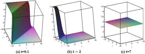
In Figure 1 we examined how the kink wave profile for $u_2(x,y,z,t)$ changed over time. At t = 2, the waves get smaller and then become stable t = 7.

Figure 1. 3D annihilation forms of a kink-wave profile with $c_1=c_2=c_3=c_4=c_5=1$ and z = 1 for $u_2(x,y,z,t)$.

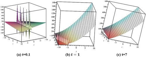
In Figure 2 as time passes, the annihilation of a multi-soliton for $u_3(x,y,z,t)$ has been observed. After t = 7, the multisoliton shape is converted into a stable wave profile.

Figure 2. 3D annihilation forms of a multi soliton profile with x = 1,$a_0=1$,$\mu =-1$ and d = 0.7 for $u_3(x,y,z,t)$.

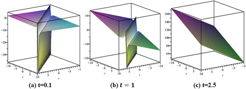
In Figure 3 we observed the stabilization of the king-bright profile over time.

Figure 3. 3D annihilation forms of a king-bright profile with A = 1,$a_0=1$,$\mu =1$ and z = 0.3 for $u_4(x,y,z,t)$.

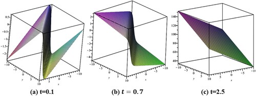
In Figure 4 another kink wave profile was seen in a similar way and was stable at t = 2.5.

Figure 4. 3D annihilation forms of a kink-wave profile with $a_0=1$, $\mu =-5$, d = 4 and z = −1 for $u_5(x,y,z,t)$.

In this work, using the WTC Kruskal algorithm, we examined the Painlavé property of the (3+1) dimensional NHB equation. We have demonstrated that the compatibility condition does not hold at the k = 6 resonance and is not Painlevé integrable. We obtained 9-dimensional Lie symmetry algebra for Equation (3(3) $u_{yt}-u_{xxxy}-3(u_x{u}_y{)}_x-3u_{xx}+3u_{zz}=0.$(3) ). We reduced the NHB equation to the ODE using some generators and their combination.Then we obtained the exact group invariant solutions of the NHB equation using Bernoulli sub-ODE, ${\displaystyle \frac{1}{G^{\mathrm{\prime }}}}$ and modified Kudryashov methods. Lie symmetry analysis of many important equations has been studied in the literature, but as a result of our research, we have seen that the symmetry analysis of the NHB has not been studied before. For this reason, we believe that our results are new, useful and different from the solutions available in the literature. On the other hand, we have provided that Equation (3(3) $u_{yt}-u_{xxxy}-3(u_x{u}_y{)}_x-3u_{xx}+3u_{zz}=0.$(3) ) is quasi-self- adjoint and for each Lie point generator we get local conservation laws via Ibragimov's nonlocal conservation method. In future works, we plan to discuss non-classical symmetries and the relationships between symmetries and conservation laws.

Disclosure statement

No potential conflict of interest was reported by the author(s).

Correction Statement

This article has been corrected with minor changes. These changes do not impact the academic content of the article.

References

- https://study.com/academy/lesson/shallow-water-waves-definition-speed-calculation.html.
- Tanwar DV, Kumar M. On Lie symmetries and invariant solutions of Broer–Kaup–Kupershmidt equation in shallow water of uniform depth. J Ocean Eng Sci. 2022. DOI:10.1016/j.joes.2022.04.027
- Ma WX. Soliton solutions by means of Hirota bilinear forms. Partial Differ Equ Appl Math. 2022;5:100220.
- Guo B, Ling L, Liu QP. Nonlinear Schrödinger equation: generalized Darboux transformation and rogue wave solutions. Phys Rev E. 2012;85(2):026607.
- Musette M. Painlevé analysis for nonlinear partial differential equations. In: Conte R, editor. The Painlevé property, one century later, CRM Series in Mathematical Physics. New York (NY): Springer; 1999. p. 517–572.
- Olver PJ. Applications of Lie groups to differential equations. Vol. 107. New York: Springer Science & Business Media; 2000.
- Tariq KU, Bekir A, Zubair M. On some new travelling wave structures to the (3+1)-dimensional Boiti-Leon-Manna-Pempinelli model. J Ocean Eng Sci. 2022. DOI:10.1016/j.joes.2022.03.015
- Alam MN, Tunç C. New solitary wave structures to the (2+1)-dimensional KD and KP equations with spatio-temporal dispersion. J King Saud Univ Sci. 2020;32(8):3400–3409.
- Islam S, Alam M, Al-Asad M, et al. An analytical technique for solving new computational? Solutions of the modified Zakharov-Kuznetsov Equation arising in electrical engineering. J Appl Comput Mech. 2021;7(2):715–726.
- Alam MN, Tunç C. The new solitary wave structures for the (2+1)-dimensional time-fractional Schrodinger equation and the space-time nonlinear conformable fractional Bogoyavlenskii equations. Alexandria Eng J. 2020;59(4):2221–2232.
- Alam MN, Tunç C. Constructions of the optical solitons and other solitons to the conformable fractional Zakharov–Kuznetsov equation with power law nonlinearity. J Taibah Univ Sci. 2020;14(1):94–100.
- Ali A, Seadawy AR, Lu D. New solitary wave solutions of some nonlinear models and their applications. Adv Differ Equ. 2018;2018(1):1–12.
- Gao LN, Zhao XY, Zi YY, et al. Resonant behavior of multiple wave solutions to a Hirota bilinear equation. Comput Math Appl. 2016;72(5):1225–1229.
- Lü X, Ma WX. Study of lump dynamics based on a dimensionally reduced Hirota bilinear equation. Nonlinear Dyn. 2016;85(2):1217–1222.
- Wang C. Lump solution and integrability for the associated Hirota bilinear equation. Nonlinear Dyn. 2017;87(4):2635–2642.
- Gao LN, Zi YY, Yin YH, et al. Bäcklund transformation, multiple wave solutions and lump solutions to a (3+1)-dimensional nonlinear evolution equation. Nonlinear Dyn. 2017;89(3):2233–2240.
- Dong MJ, Tian SF, Yan XW, et al. Solitary waves, homoclinic breather waves and rogue waves of the (3+1)-dimensional Hirota bilinear equation. Comput Math Appl. 2018;75(3):957–964.
- Zeynel M, Yasar E. A new (3+1) dimensional Hirota bilinear equation: periodic, rogue, bright and dark wave solutions by bilinear neural network method. J Ocean Eng Sci. 2022. DOI:10.1016/j.joes.2022.04.017
- Ibragimov NH. A new conservation theorem. J Math Anal Appl. 2007;333(1):311–328.
- Xu GQ, Li ZB. Symbolic computation of the Painlevé test for nonlinear partial differential equations using Maple. Comput Phys Commun. 2004;161(1-2):65–75.
- Weiss J, Tabor M, Carnevale G. The Painlevé property for partial differential equations. J Math Phys. 1983;24(3):522–526.
- Hereman W, Göktaş Ü, Colagrosso MD, et al. Algorithmic integrability tests for nonlinear differential and lattice equations. Comput Phys Commun. 1998;115(2-3):428–446.
- Lou SY, Chen CL, Tang XY. (2+ 1)-dimensional (M+ N)-component AKNS system: Painlevé integrability, infinitely many symmetries, similarity reductions and exact solutions. J Math Phys. 2002;43(8):4078–4109.
- Zhang SL, Wu B, Lou SY. Painlevé analysis and special solutions of generalized Broer–Kaup equations. Phys Lett A. 2002;300(1):40–48.
- Kumar S, Ma WX, Kumar A. Lie symmetries, optimal system and group-invariant solutions of the (3+1)-dimensional generalized KP equation. Chin J Phys. 2021;69:1–23.
- Wang G, Vega-Guzman J, Biswas A, et al. (2+1)-dimensional Boiti–Leon–Pempinelli equation–domain walls, invariance properties and conservation laws. Phys Lett A. 2020;384(10):126255.
- Jadaun V, Kumar S. Symmetry analysis and invariant solutions of (3+1)-dimensional Kadomtsev–Petviashvili equation. Int J Geom Methods Mod Phys. 2018;15(08):1850125.
- Velan MS, Lakshmanan M. Lie symmetries and invariant solutions of the shallow-water equation. Int J Non Linear Mech. 1996;31(3):339–344.
- Sadat R, Kassem M. Explicit solutions for the (2+1)-dimensional Jaulent–Miodek equation using the integrating factors method in an unbounded domain. Math Comput Appl. 2018;23(1):15.
- Ali MR, Sadat R. Lie symmetry analysis, new group invariant for the (3+1)-dimensional and variable coefficients for liquids with gas bubbles models. Chin J Phys. 2021;71:539–547.
- Ibragimov NH. Nonlinear self-adjointness and conservation laws. J Phys A: Math Theor. 2011;44(43):432002.
- Steeb WH, Euler N. Nonlinear evolution equations and Painlevé test. Singapore: World Scientific; 1988.
- Roy-Chowdhury AK. Painlevé analysis and its applications. Vol. 105. Boca Raton (USA): CRC Press; 1999.
- Adem AR, Khalique CM, Biswas A. Solutions of Kadomtsev–Petviashvili equation with power law nonlinearity in 1+3 dimensions. Math Methods Appl Sci. 2011;34(5):532–543.
- Yang H, Liu W, Yang B, et al. Lie symmetry analysis and exact explicit solutions of three-dimensional Kudryashov–Sinelshchikov equation. Commun Nonlinear Sci Numer Simul. 2015;27(1–3):271–280.
- Yong X, Chen Y, Huang Y, et al. Lie symmetry analysis for a generalized Conde-Gordoa-Pickering equation via equivalence transformations. Chin J Phys. 2020;66:430–435.
- Liu YK, Li B. Nonlocal symmetry and exact solutions of the (2+1)-dimensional Gardner equation. Chin J Phys. 2016;54(5):718–723.
- Ali MR, Ma WX. New exact solutions of Bratu Gelfand model in two dimensions using Lie symmetry analysis. Chin J Phys. 2020;65:198–206.
- Kumar S, Kumar D, Wazwaz AM. Group invariant solutions of (3+1)-dimensional generalized B-type Kadomstsev Petviashvili equation using optimal system of Lie subalgebra. Phys Scr. 2019;94(6):065204.
- Kumar S, Nisar KS, Kumar A. A (2+1)-dimensional generalized Hirota–Satsuma–Ito equations: lie symmetry analysis, invariant solutions and dynamics of soliton solutions. Res Phys. 2021;28:104621.