Investigation of possible effect of cemeteries on groundwater

Abstract

Groundwater, a vital source of fresh water for many, has been negatively impacted by human activities, climate change, and poor management. Human remains from cemeteries can contribute significantly to groundwater pollution if there is a potential connection between the cemetery and the underlying aquifer. This study aimed to assess the impact of cemeteries on groundwater using piecewise differentiation to derive decay models and numerical simulations. The results confirmed observations, and in the unlikely event of a connection between the cemetery and the underlying groundwater, each body could be considered a source of groundwater pollution. The concept of piecewise differentiation was used to provide piecewise advection-dispersion equations, and numerical simulations were presented.

KEYWORDS:

• Pollution
• cemeteries
• decay process
• mathematical models
• data analysis
• groundwater transport

1. Introduction

From the early twentieth century, the discovery and development of groundwater resources were the main focus of groundwater science. However, as irrigation, industry, and more significant engineered projects have grown, groundwater's engineering and environmental aspects have become increasingly important. Groundwater accounts for approximately 30% of all available freshwater, supporting human health, economic development, and ecological diversity [1]. Growing urbanization and the rise in population have contributed to groundwater contamination in numerous regions of the world due to the mismanagement of groundwater resources and the discharge of domestic and industrial sewage into the groundwater system. Groundwater contamination has become a significant concern due to the health risks connected with its use as drinking water. Hydrogeological analyses of aquifer water supplies have been carried out during the past 20 years. Still, as concerns about water quality have increased, predicting how contaminants will move through the subsurface environment has become vital. According to [2], groundwater contaminant migration mainly occurs through seepage, which, as shown in Figure 1, is caused by both molecular diffusion and advection–dispersion in the pore medium. The geographical, geological, and climatic factors all impact groundwater flow.

Figure 1. Main processes that occur in an aquifer. Obtained from [3].

The distribution of hydraulic conductivity in the rocks and the layout of the water table affect how the groundwater flows as a result. In cemeteries, groundwater is created as water seeps through the ground surface and travels vertically to the water table. The waters that percolate through cemeteries will carry some components of the buried remains. To characterize the mechanisms of groundwater contamination in cemeteries, the primary framework of mathematical models has to be created, and to choose an appropriate mathematical model, one must take into account the diversity of geology and hydrogeology that are present for different cemetery sites as they have a significant influence the potential impacts of any dissolved materials that migrate into the environment. The interest in understanding and modelling the exchange between irregular flows and movements of pollution within geological formations is a long-standing issue that is still not fully understood and for which a complete set of equations is still lacking. Over the past ten years, various approaches to capture nonlocalities have been put forth, such as differential operators with power laws, exponential decay, and the generalized Mittag-Leffler function. It was noted that although standard differentiation and integration models have been applied to several issues, they are unable to explain mechanisms exhibiting nonlocality behaviours [4]. The generalized Mittag-Leffler functions and exponential decay were the only ones recognized to have crossover properties, capturing the decomposition process; both had the drawback of pinpointing the precise moment and location at which crossover takes place.

In this research, we sought to derive an accurate model that might be utilized to identify pollution originating from cemeteries. In this research, we sought to derive a precise model that might be used to identify pollution originating from cemeteries and its flow and migration within a geological formation. Initially, we establish a basic decay model that illustrates the breakdown of flesh without a skeleton. Next, we run a numerical simulation to account for the environmental climate at the decay site. Then, under temperature settings, we use piecewise differentiation to examine the various degradation phases. A fractional behaviour mathematical model of the human body's aging process is presented. The model captures the crossover from a stretched exponential to a power behaviour, displaying a nonlocal character of fractional decay. Afterward, we examined the degradation process, which exhibits fractional and classical behaviour. Following our discovery of the processes by which the human body breaks down and contaminates its surroundings, we run numerical simulations and make assumptions. Our proposed groundwater transport model, referred to as the advection–dispersion equation, is based on the following assumptions: to simulate it, we first convert the human body's mass to its initial concentration.

1. We assume a single grave burial and no retention factor in geological formations.

2. We consider solitary grave burial and retention factors in geological formations.

3. We presume that two bodies can fit in the grave.

2. Impact of cemeteries on the environment and public health

Numerous research on the effects of graves on groundwater have been conducted in various locations, at multiple times, and with different environmental factors. The decomposition of human bodies emits gases like carbon dioxide and ammonia, as well as bacteria that seep into the soil and reach the groundwater, which significantly negatively influences the ecosystem. Due to the lack of knowledge on the makeup of their degradation products, the decomposition of the coffin also affects the environment. The decomposition of human bodies causes a saline contamination plume that gradually spreads below burial sites in the path of the hydraulic gradient. The dispersion of this plume is based on many dynamics, namely characteristics of the source of contamination, infiltrating rainfall, hydraulic conductivity, and the water table [5]. The effects of cemeteries on the environment are linked to the contamination of the soil, surface water, and groundwater, as well as the emission of odours when the earth above the grave is porous to gases or when the condition of burial vaults or chambers is unsatisfactory. Cemeteries in warm, humid regions like RSA and Brazil have the most significant contamination indexes [6]. A cemetery in Ditengteng, South Africa, north of Tshwane [7] discovered considerable chemical and microbiological contamination of shallow groundwater and elevated quantities of iron and manganese. In 2009, 114 monitoring sites for groundwater in Brussels, Belgium, reported the presence of nitrate, which was concentrated within a 500-meter radius near cemeteries. Active artesian wells for human and industrial use were used to get the results [8]. The findings of the [9] analysis of the presence of heavy metals such as copper, zinc, iron, and lead in the soil of the cemetery in Zandfonteim, South Africa, indicated a rise in the heavy metal as a result of the cemetery. When [10] examined soil samples from a cemetery in northwest Ohio, they looked for potentially harmful pollution levels. The study found a sharp rise in arsenic, indicating pollution from graveyard leachates. Most of the shallow aquifers formed in sand-grade (or coarser) alluvial, aeolian, or glacial deposits where burial grounds are located are contaminated. Human remains decay produces leachate, a liquid containing microorganisms, which causes groundwater contamination in cemeteries [11]. The minerals released during human decomposition could spread into the soils nearby, seep out of the graves, and contaminate the groundwater, posing a health danger to anyone living near the cemetery [12]. Claim that given the lack of a thorough investigation into the role that decomposing bodies play in the contamination of groundwater, the transmission of dangerous chemicals, and the transmission of infectious diseases, the pollution risk posed by an improperly situated cemetery is just as serious as that posed by a wrongly situated landfill [13].

High-ranking officials and experts have noticed that cemeteries harm drinking water quality. Therefore, additional studies must be done and generated to decrease and prevent groundwater contamination linked to cemetery contamination. Due to poor urban planning and a lack of accessible space, homes are often built next to cemeteries, which poses significant health risks to people [14]. International cooperation is required to advance research that considers varied environmental factors and enables method standardization. Additional investigation is needed to evaluate contamination evidence, such as amino acids, chemical compounds, formaldehyde, and arsenic.

3. Mathematical models

3.1. Decomposition of flesh model

This section will present a simple decay model depicting the decomposition of flesh without a skeleton.

Let:

$m(0)$Be the mass before the decay.

$m(t)$Be mass at a time “t”.

From the observation, we know that. (1) $\begin{array}{r}\{\begin{array}{l}{m}^{\mathrm{\prime }}(t)=-\mathrm{\lambda m}(t)\\ m(0)=m_0\end{array}\end{array}$(1) Which has a solution (2) $\begin{array}{r}m(t)=m(0)\exp (-\mathrm{\lambda t})\end{array}$(2) Where λ is the decay rate, which accounts for the climatic property of the environment where the decay occurs. In the subsurface environment, the transport of contaminants is governed by physical, chemical, and microbiological processes that occur in the soil, which are influenced by soil temperature [15]. The amount of rainfall, seasonal variations in the temperature of the surrounding air, type of soil, depth in the earth, and incident solar radiation all affect the temperature of the soil, which changes from month to month. We will present below numerical simulations in different weather conditions.

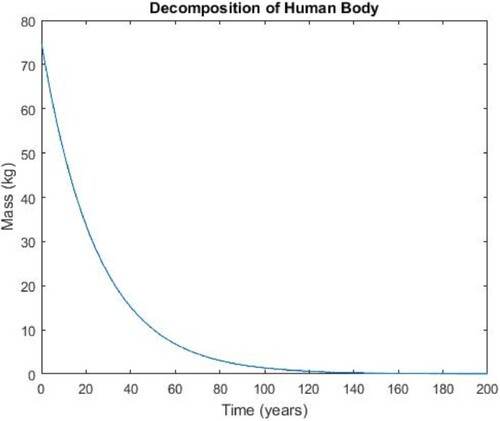
During the winter and autumn seasons, the average temperature of the soil rises as its depth increases. The decrease influences this temperature change in air temperature, which can significantly impact the soil. Temperature variations in colder climates control the frequency of freeze–thaw cycles, which can damage soil microorganisms, release nutrients, and accelerate the pace at which nitrogen breaks down and mineralizes [16]. In this case, we chose $\lambda =0.04$Moreover, I obtained the following Figure 2.

Figure 2. Decomposition of the human body in winter.

Seasonal variations in the soil temperature deep below the surface are far more minor than those in the air and occur much later because of the much higher heat capacity of soil compared to air, as well as the thermal insulation offered by plants and surface soil layers [17]. As soil depth increases, mean soil temperature decreases in spring and summer. As a result, in the spring, the soil often heats less quickly than the air and cools down by summer to act as a natural heat sink for structures. In this case, we chose $\lambda =$ She, moreover, obtained the following Figure 3.

Figure 3. Decomposition of the human body in summer.

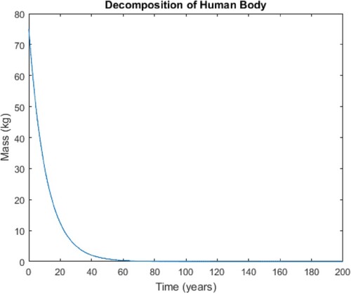
Climate factors, such as temperature, moisture content, and insect accessibility, affect how long a body decomposes. These figures illustrate the pace at which breakdown occurs at various temperature ranges. Humidity and temperature impact how quickly human bodies decompose in the winter. The human body breaks down more rapidly in summer than in winter. The simple decay model incorrectly suggests that the skeleton decomposes quickly in the human body. This model does not represent the precise breakdown of the human body into its skeleton. Skeletons break down far more slowly and take years.

3.2. Decay process with two decays

The basic decay model has been modified using piece-wise modelling techniques to demonstrate the transition of the human body breaking down under various weather conditions (seasons). The mathematical model presents two decay mechanisms. Figures 4–8 show the numerical simulations run under various weather conditions and decomposition rates.

Figure 4. Decay process when${\lambda }_1=0.05\mathrm{and}{\lambda }_2=0.09$.

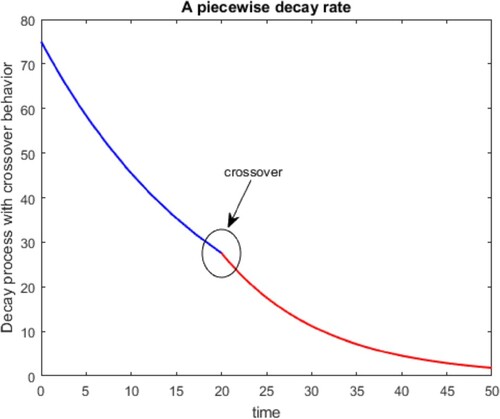
Figure 5. Decay process when ${\lambda }_1=0.09\mathrm{and}{\lambda }_2=0.05$.

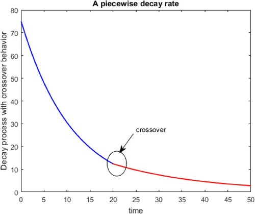
Figure 6. Decay Process when ${\lambda }_1=0.03\mathrm{and}{\lambda }_2=0.1$.

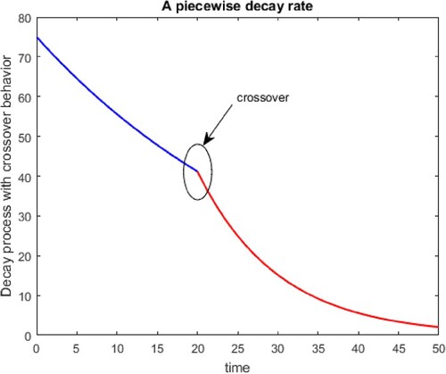
Figure 7. Decay process when ${\lambda }_1=0.1\mathrm{and}{\lambda }_2=0.01$.

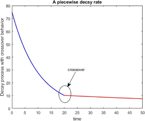
Figure 8. Decay process when ${\lambda }_1=0.1\mathrm{and}{\lambda }_2=0.01$.

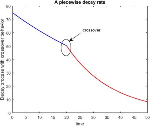
If there is a crossover behaviour in temperature during the period of decay, we will choose. $\lambda =\{\begin{array}{l}{\lambda }_1\mathrm{if}0\le t\le t_1\\ {\lambda }_2\mathrm{if}{t}_1\le t\le t_2\end{array}$If the decay is piecewise, we shall have $\lambda ={\lambda }_1\mathrm{if}0\le t\le t_1$ and $\lambda ={\lambda }_2\mathrm{if}{t}_1\le t\le T$. Therefore, the mathematical model will be given as follows: (3) $\begin{array}{r}\{\begin{array}{l}{m}^{\mathrm{\prime }}(t)=-{\lambda }_{1}m(t)\mathrm{if}0\le t\le t_1\\ m^{\mathrm{\prime }}(t)=-{\lambda }_{2}m(t)\mathrm{if}{t}_1\le t\le t_2\\ m(0)=m_0\end{array}\end{array}$(3) The above system can be solved using the Laplace transform, (4) $\begin{array}{r}m(t)=\{\begin{array}{l}m(0)\exp (-{\lambda }_{1}t)\mathrm{if}0\le t\le t_1\\ \mathrm{cexp}(-{\lambda }_{2}t)\mathrm{if}{t}_1\le t\le t_2\\ m(0)=m_0\end{array}\end{array}$(4) At $t=t_1$, we have $\begin{array}{rl}m(t_1)& =m(0)\exp (-{\lambda }_1{t}_1)=\mathrm{Cexp}(-{\lambda }_2{t}_1)\end{array}$ $\begin{array}{rl}c& =m(0)\exp (({\lambda }_2-{\lambda }_1)t_1)\end{array}$Thus, (5) $\begin{array}{r}m(t)=\{\begin{array}{l}m(0)\exp (-{\lambda }_{1}t)\mathrm{if}0\le t\le t_1\\ m(0)\exp (({\lambda }_2-{\lambda }_1)t_1)\\ \exp (-{\lambda }_{2}t)\mathrm{if}{t}_1\le t\le t_2\end{array}\end{array}$(5) The figures below illustrate the solution above:

Decomposition rates are accelerated or slowed as a body breaks down and the weather changes. The mathematical model captures the changes from one state to another with two decay processes based on the figures. This shift occurs at the boundary known as the crossover point when the weather turns from warm to cold or vice versa. However, not all of the stages of the human body's breakdown can be seen in this model.

3.3. Decomposition of the human body with fractional behaviour

Decomposition occurs in five stages: autolysis, bloating, advanced decay, active decay, and skeletonization. In this section, we will introduce a mathematical model that can be used to simulate the human body's aging process. In this instance, three different kinds of decay are observable. In the first, a rapid breakdown is brought on by the presence of flesh, blood, and water. The deterioration of tissues, hair, and skin comes in second, and the highly gradual deterioration of bones comes in last. There is crossover behaviour. Power decay occurs in the latter half, while exponential decay occurs in the first. This process exhibits a fractional decay of a nonlocal nature. The Mittag-Leffler function can capture the crossover from a stretched exponential to a power behaviour. In this case, we can assume the following fractional model: (6) $\begin{array}{r}\{\begin{array}{l}{}_0^C{D}_t^{\alpha }m(t)=-\mathrm{\lambda m}(t)\\ m(0)=m_0\end{array}\end{array}$(6) The solution is given by (7) $\begin{array}{r}m(t)=m(0)E_{\alpha }(-\lambda t^{\alpha })\end{array}$(7) The above solution can be obtained using the Laplace transform and the convolution theorem. The numerical simulation is presented below for different fractional orders Figure 9.

Figure 9. Fractional decay for different values of alpha.

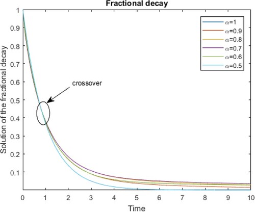
It is essential to consider the crossover as described. It is worth noting that there is a value. $t_0$ such that $0<\alpha \le 1$. The Mittag-Leffler function effectively explains how the decay follows a stretched exponential pattern, and there is a long-range dependency, which is the effect of power law.

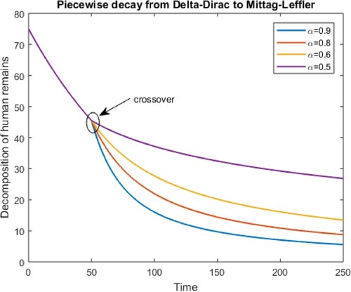
3.4. Piecewise decay from Delta-Dirac to Mittag-Leffler

This section will analyze a decay process that follows classical and fractional behaviours. We will assume that the mass is derived in a classical way between $0\le t\le t_1$ and then, in a fractional way, between $t_1\le t\le T$. The mathematical model associated with this is given below: (8) $\begin{array}{r}\{\begin{array}{l}{m}^{\mathrm{\prime }}(t)=-\mathrm{\lambda m}(t)\mathrm{if}0\le t\le t_1\\ {}_0^C{D}_t^{\alpha }m(t)=-\mathrm{\lambda m}(t)\mathrm{if}{t}_1\le t\le T\end{array}\end{array}$(8) As we did before, the solution can be obtained via the Laplace transform as (9) $\begin{array}{r}m(t)=\{\begin{array}{l}m(0)\exp (-\mathrm{\lambda t})\mathrm{if}0\le t\le t_1\\ c{E}_{\alpha }(-\lambda t^{\alpha })\mathrm{if}{t}_1\le t\le t_2\end{array}\end{array}$(9) When $t=t_1$, we have $\begin{array}{rl}m(t_1)& =m(0)\exp (-\lambda t_1)=c{E}_{\alpha }(-\lambda {t_1}^{\alpha })\end{array}$ $\begin{array}{rl}c& =m(0)\frac{\exp (-\lambda t_1)}{E_{\alpha }(-\lambda {t_1}^{\alpha })}\end{array}$Therefore, the solution is given as (10) $\begin{array}{r}m(t)=\{\begin{array}{l}m(0)\exp (-\mathrm{\lambda t})\mathrm{if}0\le t\le t_1\\ m(0){\displaystyle \frac{\exp (-\lambda t_1)}{E_{\alpha }(-\lambda {t_1}^{\alpha })}}{E}_{\alpha }(-\lambda t^{\alpha })\mathrm{if}{t}_1\le t\le T\end{array}\end{array}$(10) Where, $E_{\alpha }(-\lambda t^{\alpha })=\sum _{t=0}^{\mathrm{\infty }}\frac{{(-\lambda t^{\alpha })}^j}{\tau (\mathrm{\alpha j}+1)}$

The numerical simulation of piecewise decay from Delta-Dirac to Mittag-Leffler for different alpha values is presented below Figure 10.

Figure 10. Piecewise decay from Delta-Dirac to Mittag-Leffler for different values of alpha.

4. Numerical solutions and predictions

The first step in this section is to determine the mass of human remains that will go into the geological formation during the decay process. Theoretically, one will return to the graphs presented in the previous section to determine when the long-range starts, corresponding to the beginning of bone decay. To obtain the total mass that could contaminate the groundwater, we propose the following formula: $m_g=m(0)-m(t_c)$Where $t_c$ is the crossover time when the decomposition bone starts and $m(t_c)$ is the initial mass of skeletons, which is obtained when the flesh, water, and blood are completely decomposed.

When the total mass is identified, this mass is converted to an initial concentration that will be later used as the initial concentration for the advection–dispersion equation. In this section, we shall present some analysis that can be done to determine the migration of the deposited mass within the geological formation. This will be done according to the grave type and the geological formation's structure.

(1) If the geological formation has no retention factor and the grave only takes one body, there will be no further use of the grave. In this case, one will select the simple advection–dispersion equation as presented below: $\{\begin{array}{l}{\displaystyle \frac{\mathrm{\partial }C(x,t)}{\mathrm{\partial }t}}=D{\displaystyle \frac{{\mathrm{\partial }}^{2}C(x,t)}{\mathrm{\partial }{x}^2}}-v{\displaystyle \frac{\mathrm{\partial }C(x,t)}{\mathrm{\partial }x}}\\ C(x,0)=g(x)\\ C(0,t)=f(t)\end{array}$Where $g(x)$ and $f(x)$Re chosen accordingly.

The above equation has an exact, well-known solution available in the literature. The same solution to such an equation is given below. $\begin{array}{rl}C(x,t)& =\frac{C_0\exp [-\mathrm{\gamma t}]}{2}\{\exp \left(x\frac{q_r-u_r}{2D_r}\right)\mathrm{erfc}\left(\frac{x-u_{r}t}{2\sqrt{D_{r}t}}\right)\\ & +\exp \left(x\frac{q_r+u_r}{2D_r}\right)\mathrm{erfc}\left(\frac{x+u_{r}t}{2\sqrt{D_{r}t}}\right)\}\end{array}$Where $C_0$Is the initial concentration and $\mathrm{erfc}$Is the complementary error function given by $\mathrm{erfc}(x)=\frac{2}{\sqrt{\pi }}\underset{x}{\overset{\mathrm{\infty }}{\int }}{e}^{-t^2}\mathrm{dt}$Where $x$It can be an actual number or serial number Figures 11–15.

Figure 11. Numerical simulation in space and time.

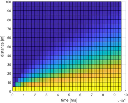
Figure 12. Numerical simulation of concentration versus distance.

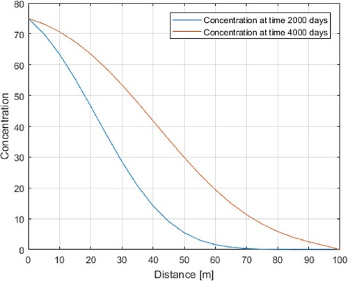
Figure 13. Numerical simulation in xyz direction.

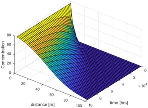
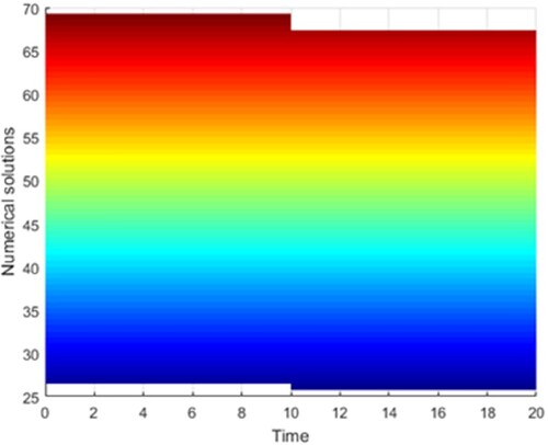
Figure 14. Numerical simulation of concentration in time.

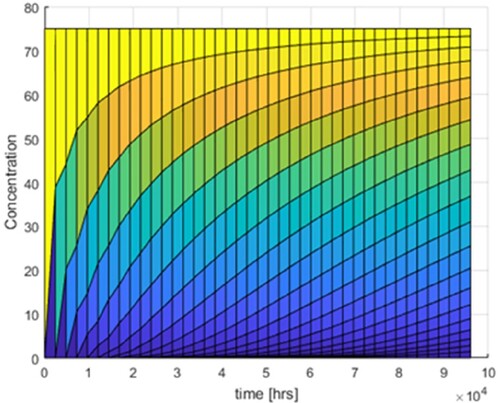
Figure 15. Numerical simulation in yz direction.

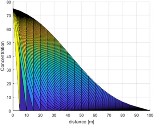
Figure 16. Numerical simulation of concentration versus distance.

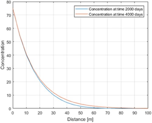
Figure 17. Numerical simulation of concentration versus distance.

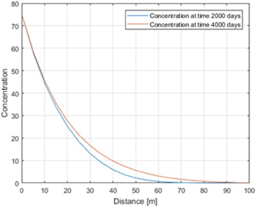
Figure 18. Numerical simulation in space and time.

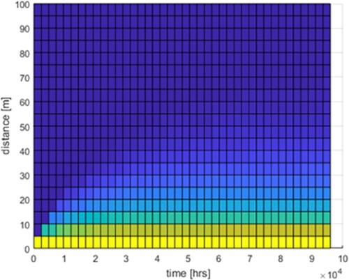
Figure 19. Numerical simulation in space and time.

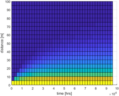
Figure 20. Numerical simulation in XYZ direction.

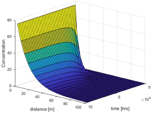
Figure 21. Numerical simulation in XYZ direction.

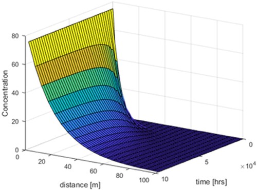
Figure 22. Numerical simulation of concentration in time.

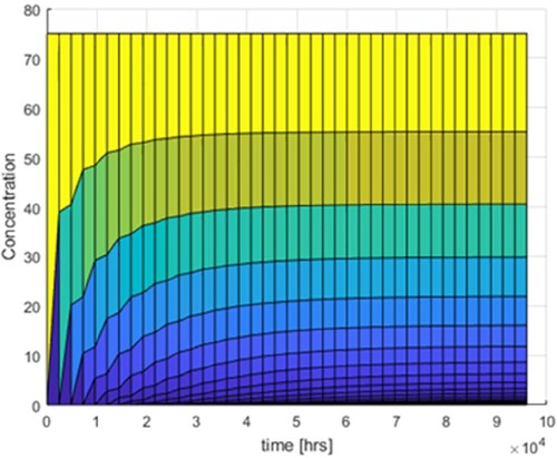
Figure 23. Numerical simulation of concentration in time.

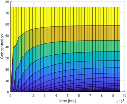
Figure 24. Numerical simulation in yz direction.

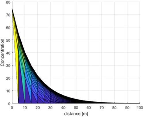
Figure 25. Numerical simulation in yz direction.

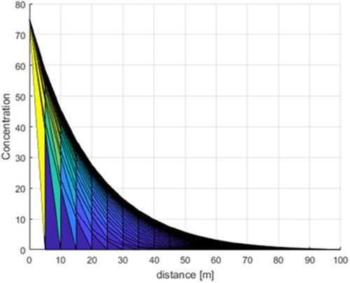
(2) If the geological formation has a retardation property and the grave can only welcome one body and further burial will not take place, the mathematical model associated with this is given below: $\{\begin{array}{l}{\displaystyle \frac{\mathrm{\partial }C(x,t)}{\mathrm{\partial }t}}=D{\displaystyle \frac{{\mathrm{\partial }}^{2}C(x,t)}{\mathrm{\partial }{x}^2}}-v{\displaystyle \frac{\mathrm{\partial }C(x,t)}{\mathrm{\partial }x}}+\mathrm{RC}(x,t)\\ C(x,0)=g(x)\\ C(0,t)=f(t)\end{array}$Where $R$Is the retardation factor.

The above equation has a well-known exact solution, and the corresponding numerical simulation as a function of the retardation factor is given below Table 1:

Table 1. Numerical simulation of retardation when R = 0.095 (left) and R = 0.070 (right).

Figure 16	Figure 17
Figure 18	Figure 19
Figure 20	Figure 21
Figure 22	Figure 23
Figure 24	Figure 25

The numerical simulations are presented in figures above 12 and 25. In this simulation, we have considered the following theoretical parameters: The initial concentration was set to be 75.T = 4000*24; [hrs] total time, D = (1$E^{-6}$)*3600; [m²/hr] dispersion constant, V = (1$E^{-7}$)*3600; [m/hr] velocity, L = 100; [m] Total length N = 20; a spatial grid sections, M = 40 temporal grid sections, dx = L/N; spatial spacing, dt = T/M; time spacing, C(1,:) = 75; inlet concentration set to 100 for all time; and for the case of retardation factor, we have chosen R = 0.095 and 0.07.

(3) Now we shall assume that the grave can accommodate two bodies, i.e. from time $t_1$ to time$t_2$, The first body is decomposed, and the initial concentration is obtained as$m_1$. Then, after the waiting period of$t_w$, Another body is placed, releasing a total mass of$m_2$, And this happened between $t_3$and$t_4$. With no retardation factor, the following mathematical model is presented: $\{\begin{array}{l}{\displaystyle \frac{\mathrm{\partial }C(x,t)}{\mathrm{\partial }t}}=D{\displaystyle \frac{{\mathrm{\partial }}^{2}C(x,t)}{\mathrm{\partial }{x}^2}}-v{\displaystyle \frac{\mathrm{\partial }C(x,t)}{\mathrm{\partial }x}}\\ C(0,t)=g(t)\mathrm{if}0\le t\le t_1\\ C(x,0)=f(x)\\ \begin{array}{l}C(x,0)=f(x)\\ {\displaystyle \frac{\mathrm{\partial }{C}_1(x,t)}{\mathrm{\partial }t}}=D{\displaystyle \frac{{\mathrm{\partial }}^2{C}_1(x,t)}{\mathrm{\partial }{x}^2}}-v{\displaystyle \frac{\mathrm{\partial }{C}_1(x,t)}{\mathrm{\partial }x}}\end{array}\\ \begin{array}{l}{C}_1(0,t)=g^{{}^{\mathrm{\prime }}}(t)\mathrm{if}{t}_{\mathrm{waiting}}\le t\le \mathrm{\infty }\\ C_1(x,t_{\mathrm{waiting}})=f(x)\end{array}\\ C_1(x,t_{\mathrm{waiting}})=f(x)\end{array}$The numerical simulations of the above equation are presented below Figures 26–29:

Figure 26. Solution of advection-dispersion in space.

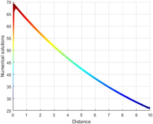
Figure 27. Numerical solution of concentration over time.

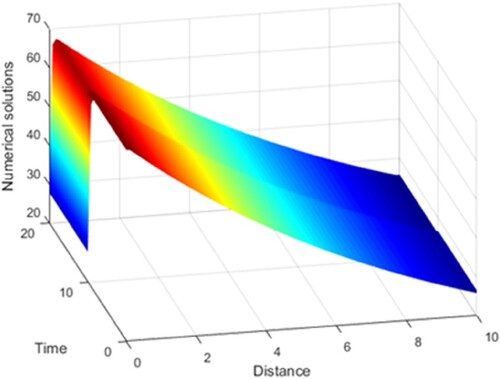
Figure 28. Advection-dispersion solution in space and time.

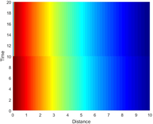
Figure 29. Numerical solution of advection-dispersion in xyz direction.

However, if there is a retardation factor, the following mathematical model is provided: $\{\begin{array}{l}{\displaystyle \frac{\mathrm{\partial }C(x,t)}{\mathrm{\partial }t}}=D{\displaystyle \frac{{\mathrm{\partial }}^{2}C(x,t)}{\mathrm{\partial }{x}^2}}-v{\displaystyle \frac{\mathrm{\partial }C(x,t)}{\mathrm{\partial }x}}+\mathrm{RC}(x,t)\\ C(0,t)=g(t)\mathrm{if}0\le t\le t_1\\ C(x,0)=f(x)\\ {\displaystyle \frac{\mathrm{\partial }{C}^{\mathrm{\prime }}(x,t)}{\mathrm{\partial }t}}=D{\displaystyle \frac{{\mathrm{\partial }}^2{C}^{\mathrm{\prime }}(x,t)}{\mathrm{\partial }{x}^2}}-v{\displaystyle \frac{\mathrm{\partial }{C}^{\mathrm{\prime }}(x,t)}{\mathrm{\partial }x}}+R{C}^{\mathrm{\prime }}(x,t)\\ C^{\mathrm{\prime }}(0,t)=g^{\mathrm{\prime }}(t)\mathrm{if}{t}_{\mathrm{waiting}}\le t\le T\\ C^{\mathrm{\prime }}(x,0)=f(x)\end{array}$Here, we have considered two initial conditions, including $C_0$ and $C_1$, Which are the initial concentrations for the first body and the second concentration for the second body. The numerical simulation shows that there is already a trace of the first concentration at the end of the waiting time. When adding the second concentration, there is a rise in concentration near the grave, and then there is a movement of waste that also follows the path of the first pollution. From this analysis, one will notice that while the reopening of graves is helpful in terms of space, they pollute the groundwater or the environment more than the classical burial, which consists of burying only one body. Several practices, such as cremation and aquamation, could serve the same purpose of reducing space usage. We can conclude that the practice of reopening graves is not safe for the environment and groundwater.

5. Conclusion

In this paper, we investigated a transport model that could forecast unusual behaviours in the movement of pollution from cemeteries. We developed some mathematical models to demonstrate how the human body breaks down under various circumstances and performed numerical analysis on the well-known advection–dispersion equation. To predict how much mass is released from the body to the geological formation, we have used a simple decay equation for a simple decomposition of flesh. This model was, however, unable to replicate crossover behaviours that show fast and slow decomposition due to flesh and bone. To solve this problem, we have used the concept of piecewise differentiation to obtain a piecewise decay model. This new model can capture the decomposition by considering the effect of temperature. To capture the crossover from stretched exponential to power law, we have introduced the notion of fractional derivatives and also extended the new model using classical and fractional derivatives. A solution of the fractional decay model, as opposed to the classic decay model with a solution exponential function, is a more precise representation of the fraction decay that reflects the breakdown of the human body. The three stages of the fractional decay solution are stretched exponential behaviour, crossover point, and power-law behaviour. The obtained results can be used to theoretically determine how much mass will be released within the geological formation. The formula to determine this was suggested. Under the condition that all mass reaches the groundwater, a methodology to verify the presence of this pollution was suggested. It was suggested that the released mass can be converted to a concentration used as the initial condition for the chosen advection–dispersion equation. The selected advection–dispersion equation can then be used to show the movement of the pollution within the geological formation. Two scenarios – the advection–dispersion equation with retardation and the advection–dispersion equation without retardation – were used to analyze the transport of contaminants within the geological formation. In MATLAB, the advection–dispersion was used to illustrate the human remains’ spread, and the equation's stability and accuracy were obtained. About the decay rate, we found that the dispersion coefficient and velocity are pretty sensitive.

Cemeteries are considered to be one of the most polluting sources. The minerals released from the burials are the primary contributors to contamination from cemeteries. The decomposition of human bodies releases gases such as carbon dioxide, ammonia, and bacteria that enter the soil and reach groundwater. Water percolates through cemeteries carrying human remains, and the variety of the hydrogeology and geology found at various cemetery sites affects the movement of these dissolved elements into the environment. The figures show that human decomposition produces a saline contamination plume that moves beneath the graves toward the hydraulic gradient. We have presented different cases; however, we conclude that the case with re-used graves is more polluting than the single-used graves, so this type should be discouraged.

Disclosure statement

No potential conflict of interest was reported by the author(s).

References

- Jha MK, Chowdhury A, Chowdary VM, et al. Groundwater management and development by integrated remote sensing and geographic information systems: prospects and constraints. Water Resour Manage. 2007;21:427–467. doi:10.1007/s11269-006-9024-4
- Shackelford CD. Contaminant transport. In: DE Daniel, editor. Geotechnical practice for waste disposal. London: Chapman and Hall; 1993.
- Talabi A, Kayode T. Groundwater pollution and remediation. J Water Resource Prot. 2019;11:1–19.
- Atangana A, Araz Sİ. New concept in calculus: piecewise differential and integral operators. Chaos Solit Fractals. 2021;145:110638.
- Franco DSP. The environmental pollution caused by cemeteries and cremations: a review. Chemosphere. 2022;307(16):136025.
- Zychowski J. Impact of cemeteries on groundwater chemistry: a review. Catena. 2012;93:29–37. doi:10.1016/j.catena.2012.01.009
- Tumagole KB. Geochemical survey of underground water pollution at Ditengteng northern cemetery in Tshwane municipality. Johannesburg: University of Johannesburg; 2009.
- Mattern S, Sebilo M, Vanclooster M. Identification of the nitrate contamination sources of the Brusselian sands groundwater body (Belgium) using a dual-isotope approach. Isot Environ Health Stud. 2011;47(3):297–315. doi:10.1080/10256016.2011.604127
- Jonker C, Olivier J. Mineral contamination from cemetery soils: a case study of Zandfontein Cemetery, South Africa. Int J Environ Res Public Health. 2012;9:511–520. doi:10.3390/ijerph9020511
- Spongberg AL, Becks PM. Inorganic soil contamination from cemetery leachate. Water Air Soil Pollut. 2000;117(1–4):313–327. doi:10.1023/A:1005186919370
- Engelbrecht JFP. An assessment of health aspects of the impact of domestic and industrial waste disposal activities on groundwater resources. Pretoria: Water Research Commission; 1993.
- Üçisik AS, Rushbrook P. The impact of cemeteries on the environment and public health. Europe: World Health Organization; 1998.
- Roux P, Page TC, Holland-Mute LM. Waste management vs mismanagement in South Africa. Johannesburg: Seminar and Workshop on Environmental waste management; 1991.
- Hariyono WP. Vertical cemetery. Procedia Eng. 2015;118:201–214. doi:10.1016/j.proeng.2015.08.419
- Pepper IL, Brusseau ML. Chapter 2 - physical-chemical characteristics of soils and the subsurface. In: ML Brusseau, IL Pepper, CP Gerba, editor. Environmental and pollution science. s.l.: Academic Press; 2019. p. 9–22.
- Wang L, D’Odorico P. Decomposition and mineralization. In: SE Jørgensen, BD Fath, editor. Encyclopedia of ecology. s.l.: Academic Press; 2008. p. 838–844.
- Gonzalez RG, Verhoef A, Vidale PL, et al. Interactions between the physical soil environment and a horizontal ground coupled heat pump for a domestic site in the UK. Renew Energ. 2012;44:141–153. doi:10.1016/j.renene.2012.01.080