Optimal multiple functional regression analysis using perturbation theory

ABSTRACT

A regression analysis is presented based on several functions. A normalized data are used which enables the usage of magnitude of orders in perturbation theory. The criteria to eliminate unnecessary base functions are derived with the aid of order of magnitudes in perturbations. The analysis generalizes the previous work on polynomial regression of arbitrary orders. Properties of the regression coefficients are outlined via theorems. Numerical tests are conducted to outline the usage of the analysis to eliminate unnecessary functions and obtain a reasonable approximation of the data in a continuous form.

KEYWORDS:

• Functional regression
• perturbation analysis
• data approximation

1. Introduction

When conducting experiments, one may obtain data (x_i, y_i) i = 1,2, … N in a discrete form. Due to the high costs of experimentation, a limited number of experiments can be conducted which displays the dependence of data in a discrete form not closely spaced. The next step is then to obtain a continuous functional relationship which is derived from the given data set and approximates the data in the given interval. A widely used method to achieve this continuous approximation task is the employment of regression analysis [1]. Linear regression is the most common method used in which a straight line best approximating the data is searched. Depending on the distribution of the data, linear approximation might not be suitable for many cases, which dictates a nonlinear functional relationship to be employed for approximation. Nonlinear regression analysis was reviewed with conceptual focus rather than the formulas by Motulsky and Ransnas [2].

One of the common methods used is to employ a polynomial type continuous function to approximate the data. The minimum highest degree of polynomial that approximates reasonably well the original data is a mathematical problem that was treated by several researchers. In Anderson’s procedure [3], a predetermined highest-order n value is selected and the procedure tests whether the coefficients vanish or not. If the highest order coefficient vanishes, one lower degree polynomial is selected and the procedure repeats itself until a non-vanishing highest degree coefficient is obtained. In a recent study [4], instead of the rather restrictive vanishing highest degree coefficient assumption of [3], a somewhat relaxed assumption which requires the coefficient of highest degree to be negligible was employed using normalized data. Within the context of perturbation theory [5], if the highest degree coefficient is small, that is of O(ϵ), ϵ<<1, then the degree of the polynomial is lowered by one. The analysis is repeated until an O(1) highest degree coefficient is obtained. For some other relevant results and implementation of the procedure due to Anderson, refer to Dette [6] and Dette and Studden [7]. For polynomial type of regressions, non-parametric regression methods were also used to test the validity of the approximation by Jayasuriya [8]. Tomašević et al. [9] employed Chebyshev polynomials in the regression analysis and lowering the degree of approximation was discussed. Ivanov and Ailuro [10] proposed a new Taylor Map Polynomial Neural Network method for high-order polynomial regressions.

In this study, the work on polynomial regression based on perturbation theory due to Pakdemirli [4] is generalized to arbitrary multiple base functions. To apply perturbation concepts, the first step is to make the data non-dimensional by dividing by the maximum values of the variables. Choosing a set of base functions to approximate the data, the regression coefficients are calculated by the derived formulas. Theorems on the properties of the coefficients as well as approximate errors may be employed as guides to remove the unnecessary functions. The elimination algorithm is discussed and the applications of the theorems are given by numerical analysis of two sets of specific data.

2. Multiple function regression

For the given data (x_i, y_i), i = 1,2, … N, an approximation in the form of a series (1) $y\left(x\right)=\sum _{k=0}^K{a}_k{f}_k\left(x\right),$(1) is assumed where $f_k\left(x\right)$ are the base functions and $a_k$ are their coefficients. The special case of the base functions $f_k\left(x\right)=x^k$ were already treated in [4]. Defining the total difference square as (2) $e^2=\sum _{i=1}^N(y_i-y\left(x_i\right){)}^2,$(2) and requiring this term to be minimum yields (3) $\frac{\mathrm{\partial }e}{\mathrm{\partial }{a}_k}=0,k=0,1,2,..K,$(3) which is the method of least squares [11]. Equations (1)–(3) lead to the below matrix equation (4) $\mathbf{\text{F}}\mathbf{\text{A}}=\mathbf{\text{Y}},$(4) where (5) $\begin{array}{rl}\mathbf{\text{F}}& =[\begin{array}{cc}\sum _{i=1}^N{f}_0^2\left(x_i\right)& \sum _{i=1}^N{f}_0\left(x_i\right)f_1\left(x_i\right)\\ \sum _{i=1}^N{f}_0\left(x_i\right)f_1\left(x_i\right)& \sum _{i=1}^N{f}_1^2\left(x_i\right)\\ :& :\\ \sum _{i=1}^N{f}_0\left(x_i\right)f_K\left(x_i\right)& \sum _{i=1}^N{f}_1\left(x_i\right)f_K\left(x_i\right)\end{array}\\ & \begin{array}{cc}\dots & \sum _{i=1}^N{f}_0\left(x_i\right)f_K\left(x_i\right)\\ \dots & \sum _{i=1}^N{f}_1\left(x_i\right)f_K\left(x_i\right)\\ \dots & :\\ \dots & \sum _{i=1}^N{f}_K^2\left(x_i\right)\end{array}]\end{array}$(5) (6) $\begin{array}{rl}\mathbf{\text{A}}& =\left[\begin{array}{c}\begin{array}{c}{a}_0\\ a_1\end{array}\\ \begin{array}{c}:\\ a_K\end{array}\end{array}\right]\end{array}$(6) (7) $\begin{array}{rl}\mathbf{\text{Y}}& =\left[\begin{array}{c}\begin{array}{c}\sum _{i=1}^N{y}_i{f}_0\left(x_i\right)\\ \sum _{i=1}^N{y}_i{f}_1\left(x_i\right)\end{array}\\ \begin{array}{c}:\\ \sum _{i=1}^N{y}_i{f}_K\left(x_i\right)\end{array}\end{array}\right].\end{array}$(7)

Solving for the optimum coefficients (8) $\mathbf{\text{A}}={\mathbf{\text{F}}}^{-1}\mathbf{\text{Y}}.$(8) The standard regression error is [11] (9) $S_{y/x}={\left[\frac{1}{N-\left(K+1\right)}\sum _{i=1}^N{\left(y_i-y\left(x_i\right)\right)}^2\right]}^{1/2},$(9) where N-(K + 1) represents the degree of freedom.

3. Theorems based on perturbations

To compare correctly the order of magnitudes of terms, it is advised to use dimensionless quantities in perturbation theory [12]. The experimental data may be cast into a dimensionless form by dividing the data by their maximum values in magnitude (10) ${\overline{x}}_i=\frac{x_i}{x_{\max }},{\overline{y}}_i=\frac{y_i}{y_{\max }},$(10) where ${\overline{x}}_i$ and ${\overline{y}}_i$are the normalized data. The dimensionless data are trapped in a square region ($-1\le {\overline{x}}_i\le 1,-1\le {\overline{y}}_i\le 1$). The theorems are applicable for a regression analysis of the normalized data. Important features of the coefficients can be deduced with the aid of normalization which cannot be retrieved using the original data.

Theorem 3.1.

For the multiple functional regression analysis of k + 1 functions using the normalized data (11) $\overline{y}\left(x\right)=\sum _{k=0}^K{a}_k{f}_k\left(\overline{x}\right),$(11) if all $a_k$ have the same sign, $f_k\left(\overline{x}\right)\sim O\left(1\right)$ and $f_k\left(\overline{x}\right)$ possess the same sign in at least a subinterval of the domain D, then $a_k\sim O\left({ϵ}^{m_k}\right),m_k\ge 0(ϵ\ll 1)$.

Proof 1:

According to the theorem, there exist no large coefficients with magnitude orders greater than 1 if the coefficients all have the same signs. Because the data are trapped in a square, $|\overline{y}\left(x\right)|\le O\left(1\right)$. From (11) with $f_k\left(\overline{x}\right)\sim O\left(1\right)$ throughout the whole domain and $f_k\left(\overline{x}\right)$ possess the same sign in at least a subinterval of the domain D, then (12) $a_0+a_1+\dots +a_K\le O\left(1\right).$(12) Inserting the orders of each term (13) $O\left({ϵ}^{m_0}\right)+O\left({ϵ}^{m_1}\right)+\dots O\left({ϵ}^{m_{K-1}}\right)+O\left({ϵ}^{m_K}\right)\le O\left(1\right).$(13) Assume that one of the $m_k$ is negative, then, there exists a large term which cannot be balanced by the same sign coefficients to yield (13) since $ϵ$ is a small parameter. Hence, if all coefficients have the same sign, the magnitudes of coefficients are O(1) or less

Theorem 3.2.

For the multiple functional regression analysis of k + 1 functions using the normalized data (14) $\overline{y}\left(x\right)=\sum _{k=0}^K{a}_k{f}_k\left(\overline{x}\right),$(14) assume that there are large coefficients i.e. $a_k\sim O\left({ϵ}^{m_k}\right),m_k<0\left(ϵ\ll 1\right)$, then the coefficients cannot possess the same signs. Other large coefficient(s) $a_j\sim O\left({ϵ}^{m_j}\right),m_j<0$, must exist with opposite signs subject to the conditions that, $f_k\left(\overline{x}\right)\sim O\left(1\right)$ throughout the whole domain and all $f_k\left(\overline{x}\right)$ possess the same sign in at least a subinterval of the domain D.

Proof 2:

Since $f_k\left(\overline{x}\right)\sim O\left(1\right)$ throughout the whole domain, all $f_k\left(\overline{x}\right)$ possess the same sign in at least a subinterval of the domain D and $\overline{y}\left(x\right)\le O\left(1\right)$ due to normalization, from (14) (15) $O\left({ϵ}^{m_0}\right)+O\left({ϵ}^{m_1}\right)+\dots O\left({ϵ}^{m_{K-1}}\right)+O\left({ϵ}^{m_K}\right)\le O\left(1\right).$(15) If a large term exists with $m_k<0$, it should be balanced by some other large term(s) $a_j\sim O\left({ϵ}^{m_j}\right),m_j<0$ with altering signs because the coefficients’ sum add to O(1)

Theorem 3.3.

For a good multiple functional regression of k + 1 functions for the normalized data (16) $\overline{y}\left(x\right)=\sum _{k=0}^K{a}_k{f}_k\left(\overline{x}\right),$(16) the regression coefficients’ sum are bounded (17) $\sum _{k=0}^K{a}_k\le O\left(1\right)$(17) subject to the conditions that, $f_k\left(\overline{x}\right)\sim O\left(1\right)$ throughout the whole domain and all $f_k\left(\overline{x}\right)$ possess the same sign in at least a subinterval of the domain D ▪

Proof 3:

Due to normalization, a good approximation should satisfy $\overline{y}\left(\overline{x}\right)\le O\left(1\right)$. Employing the given properties of the base functions (18) $\sum _{k=0}^K{a}_k\le O\left(1\right),$(18) immediately from (16). Therefore, a good regression approximation should have coefficient sums to be not larger than O(1)

Theorems 3.1–3.3 display the conditions for the regression coefficients. Excess base functions can be eliminated using these conditions. An additional theorem is given for the regression errors.

Theorem 3.4.

The bound of the standard regression error is (19) $S_{\overline{y}/\overline{x}}\le O\left({ϵ}^2\right),ϵ\ll 1,$(19) if the base functions are selected suitable to the normalized data ▪

Proof 4:

If the base functions are selected suitable, the associated data and the curve data are close to each other. Within the box of lengths O(1), the error between data and their approximation may be negligibly small compared to 1, which leads to (20) $|{\overline{y}}_i-\overline{y}\left({\overline{x}}_i\right)|\le O\left({ϵ}^2\right),ϵ\ll 1.$(20) Inserting (20) into (9) (21) $S_{\overline{y}/\overline{x}}={\left[\frac{N}{N-\left(K+1\right)}O\left({ϵ}^4\right)\right]}^{1/2}.$(21) For an admissible regression, the data N should be greater than the degrees of freedom K + 1 leading to $\frac{N}{N-\left(K+1\right)}\sim O\left(1\right)$. From (21), $S_{\overline{y}/\overline{x}}\le O\left({ϵ}^2\right)$

The above theorem gives a criterion on the suitability of the base functions in general. If the base functions are selected wrong, the error cannot be reduced to $O\left({ϵ}^2\right)$, which indicates that one has to change the base functions rather than eliminating the unnecessary ones from the set.

4. Numerical applications

The theory is applied to two specific problems. The usage of the theorems and elimination of unnecessary base functions are depicted using specific data sets.

4.1. Sample Data Set 1

In Table 1, a distorted data set which is close to the functional relationship $y=x^2$ is given. Assume that initial trial regression functions for the normalized data are selected as (22) $\overline{y}\left(\overline{x}\right)=a_0{\overline{x}}^2+a_1{\overline{x}}^3+a_2\overline{x}+a_3\sin \overline{x},$(22) with K = 3. The determinant of the coefficient matrix, the coefficients with their sum and the regression errors are given for each calculation.

Table 1. Multiple functional regression results for Data Set 1.

Data 1	x = [0 1 2 3 4 5 6 7] y = [0 1 5 9 14 25 37 49]	$\overline{x}$=[0.0000 0.1429 0.2857 0.4286 0.5714 0.7143 0.8571 1.0000] $\overline{y}$=[0.0000 0.0204 0.1020 0.1837 0.2857 0.5102 0.7551 1.0000]
K	Regression function	det(F)	ao …  … .aK	Σak	Sy/x
3	$a_0{\overline{x}}^2+a_1{\overline{x}}^3+a_2\overline{x}+a_3\sin \overline{x}$	2.88 10^−10	−0.6323	−12.0183	0.0184
			−11.7147
			82.4629
			−82.1343
2	$a_0{\overline{x}}^2+a_1{\overline{x}}^3+a_2\overline{x}$	0.0022	0.8047	1.0113	0.0212
			0.1582
			0.0484
1	$a_0{\overline{x}}^2+a_1{\overline{x}}^3$	0.0806	0.9426	1.0093	0.0196
			0.0667
0	$a_0{\overline{x}}^2$	1.9475	1.0017	1.0017	0.0189

From the table, the initial suggestion with four base functions is not appropriate. The determinant of the coefficient matrix is highly singular which indicates that the choice inherits redundant functions [4]. Inspecting the coefficients, there are extremely large coefficients (Theorem 3.2) one of which has to be eliminated. The coefficients sum is also not O(1) (Theorem 3.3) which suggests redundant base functions. The regression error is small which is admissible (Theorem 3.4) and indicates that there are at least some suitable functions within the base function set to express the data. Eliminating the $\sin \overline{x}$ term and repeating the calculations for K = 2, the determinant of the F matrix is not as singular as in the first case. All coefficients have the same sign, the largest being O(1) (Theorem 3.1). Note that the linear term coefficient is extremely small which suggests that its influence on the solution is very marginal. The sum of the coefficients is O(1) which is an indication that the regression is better than the previous one. The regression error is negligibly higher than the former case though. Results suggest that the linear term $\overline{x}$ is redundant and hence eliminated. Computations for K = 1 indicate that the determinant is not extremely small, the coefficients have the same sign and at most O(1) (Theorem 3.1), their sum are O(1) (Theorem 3.3) and the error is reduced in contrast to the previous case. The small coefficient of the cubic term suggests that it can also be eliminated resulting in the K = 0 case. For this case, the determinant is non-singular, the coefficient and sum is O(1) and the error is one of the lowest values. Hence, a simple quadratic function is sufficient to approximate the given data and there is no need for additional functions.

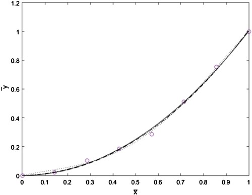
In Figure 1, the normalized data set and the approximate curves are compared. While all cases produce visually admissible continuous functions close to each other, the simplest case of K = 0 has to be selected to reduce the computations.

Figure 1. Comparison of the normalized data (o) with the regression results for K = 3 (…), K = 2(-.), K = 1 (–), K = 0 (solid).

4.2. Sample Data Set 2

In Table 2, a distorted data set which is close to the functional relationship $y=\frac{3}{1+x}+2\mathrm{sinx}$ is given. Assume that an initial trial regression function for the normalized data is selected as (23) $\overline{y}\left(\overline{x}\right)=a_0\frac{1}{1+10\overline{x}}+a_1\text{sin}\left(10\overline{x}\right)+a_2\text{cos}\left(10\overline{x}\right),$(23) with K = 2. The determinant of the coefficient matrix, the coefficients with their sum and the regression errors are given for each calculation.

Table 2. Multiple functional regression results for Data Set 2.

Data 2	x = [ 0 1 2 3 4 5 6 7 8 9 10] y = [ 3 3.2 2.8 1 -0.9 -1.4 -0.1 1.7 2.3 1.1 -0.8]	$\overline{x}$=[0.0 0.1 0.2 0.3 0.4 0.5 0.6 0.7 0.8 0.9 1.0] $\overline{y}$=[ 0.9375 1.0000 0.8750 0.3125 -0.2813 -0.4375 -0.0313 0.5313 0.7187 0.3438 -0.2500]
K	Regression function	det(F)	ao …  … .aK	Σak	Sy/x
2	$a_0\frac{1}{1+10\overline{x}}+a_1\text{sin}\left(10\overline{x}\right)+a_2\text{cos}\left(10\overline{x}\right)$	41.2046	0.9370	1.5628	0.0046
			0.6206
			0.0052
1	$a_0\frac{1}{1+10\overline{x}}+a_1\text{sin}\left(10\overline{x}\right)$	7.4421	0.9398	1.5604	0.0059
			0.6206

From the table, the initial suggestion with three base functions is not appropriate. All the coefficients have the same sign and at most O(1) (Theorem 3.1). The cosine term coefficient is extremely small that suggests elimination of the base function $\text{cos}\left(10\overline{x}\right)$. Repeating the calculations for K = 1, there is no negligible function since all coefficients are O(1), the sum is also O(1) (Theorem 3.3) and the error is small enough (Theorem 3.4). All indicators in the analysis points to an admissible regression and one has to terminate calculations at this level. If one eliminates further the sine function also, the standard regression error becomes 0.4522, a large value which is not small (Theorem 3.4) justifying that the double function approximation is the best one.

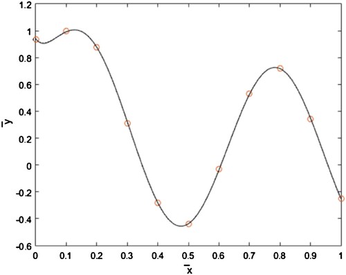
The normalized data set and the regression results are compared in Figure 2. While both cases produced visually admissible continuous functions close to each other, the simplest case of K = 1 has to be selected to reduce the computations.

Figure 2. Comparison of the normalized data (o) with the regression results for K = 2 (…), K = 1(solid).

5. Concluding remarks

For multiple function regression analysis, a theory based on perturbations is developed to test whether the selections of base functions are appropriate or not. The normalized data are used to enable a perturbational analysis. Theorems are given that aid in determining the best options for the analysis. The algorithm steps are summarized below:

1. Select an initial K + 1 trial base functions.

2. Calculate next the determinant, the coefficients with their sum and the regression error.

3. If the determinant is highly singular, then it is an indication that there are redundant base functions.

4. If the coefficients have both positive and negative signs, eliminate one of the large coefficients and the corresponding function.

5. If all the coefficients have the same signs, eliminate the extremely small ones which do not have enough contribution to the result.

6. Check the sum of the coefficients as it has to be O(1) for a good regression approximation.

7. Check the standard regression error which has to be extremely small.

8. Eliminate functions one by one until all indicators reveal an admissible approximation and use this minimum number of functions for computational simplicity.

The algorithm will definitely fail if all the initial trial base functions are not suitable at all to represent the original data. A better approximation cannot be found by the elimination process in that case. For a restricted case of polynomial regressions, refer to [4] for a similar analysis. This paper is a generalization of the previous analysis to arbitrary base functions. A future work might be to use additional parameters inside the arguments of the base functions.

Author contribution

M. P is the single author responsible for all stages of the manuscript.

Disclosure statement

No potential conflict of interest was reported by the author(s).

References

- Holman JP. Experimental methods for engineers. Tokyo: McGraw-Hill; 1978.
- Motulsky HJ, Ransnas LA. Fitting curves to data using nonlinear regression: a practical and nonmathematical review. FASEB J. 1987;1:365–374. doi:10.1096/fasebj.1.5.3315805
- Anderson TW. The choice of the degree of a polynomial regression as a multiple decision problem. Ann Math Stat. 1962;33:255–265. doi:10.1214/aoms/1177704729
- Pakdemirli M. A new perturbation approach to optimal polynomial regression. Math Comput Appl. 2016;21(1):1–8. doi:10.3390/mca21010001
- Nayfeh AH. Introduction to perturbation techniques. New York (NY): John Wiley; 1981.
- Dette H. Optimal designs for identifying the degree of a polynomial regression. Ann Stat. 1995;23:1248–1266.
- Dette H, Studden WJ. Optimal designs for polynomial regression when the degree is not known. Stat Sin. 1995;5:459–473.
- Jayasuriya BR. Testing for polynomial regression using nonparametric regression techniques. J Am Stat Assoc. 1996;91:1626–1631. doi:10.1080/01621459.1996.10476731
- Tomašević N, Tomašević M, Stanivuk T. Regression analysis and approximation by means of chebyshev polynomial. Informatologia. 2009;42:166–172.
- Ivanov A, Ailuro S. TMPNN: high-order polynomial regression based on Taylor map factorization. In: The Thirty-Eight AAAI Conference on Artificial Intelligence; 2024. p. 12726–12734. doi:10.1609/aaai.v38i11.29168
- Chapra SC, Canale RP. Numerical methods for engineers. New York (NY): Mc Graw Hill; 2014.
- Pakdemirli M. Strategies for treating equations with multiple perturbation parameters. Math Eng Sci Aerosp MESA. 2023;14(4):1–18.