Exploring the dynamics of coupled systems: fractional q-integro differential equations with infinite delay

Abstract

The objective of this study is to demonstrate the existence and uniqueness of a solution to a coupled system of infinite-delay fractional q integro-differential equations. The equation that will be the focus of this paper's analysis is noteworthy and innovative since it combines fractional differentiation with fractional q integration and has numerous applications to real-world occurrences. The existence of the solution is established using the Schauder fixed-point theorem. The uniqueness of a solution will be evaluated using Banach's fixed-point theorem. The definitions of the Riemann fractional q integral and the Caputo fractional derivative are used to arrive at a numerical solution to the coupled system. Then, the merge of the trapezoidal finite difference methodology is integrated. The finite difference approach is used for the first and second derivative components, whereas the trapezoidal method is used for the integral components. As a result, a set of straightforward algebraic equations will be produced, from which we can deduce the solution. Some applications are provided to illustrate our main conclusions.

Keywords:

• Fractional derivative
• coupled system of q-integro-differential equation
• existence and uniqueness of solution
• applications

1. Introduction

Recently, over the past few decades, delay differential equations have attracted more attention as a way to simulate real-world occurrences. Many researchers are interested in studying various integral and integro differential equations because of their many applications in real life phenomena [1–5]. There are many authors interested in studying the existence and uniqueness of a variety of differential and integro-differential equations with bounded delay and infinite delay. In Abbas [6], introduced the existence and uniqueness of delay differential equation with fractional order. In Benchohra et al. [7], discussed the existence and uniqueness of solutions for two fractional differential equations with infinite delay. In Babakhani et al. [8], studied two classes of nonlinear differential equations including Riemann-Liouville fractional derivatives with infinite delay. In Liu and Zhao [9], introduced the existence and uniqueness of a class of coupled systems of infinite delay fractional integro-differential equations. In Ravichandran and Baleanu [10], used Mönch's fixed point theorem to study the existence of solutions to integro-differential equations, including the Caputo derivative. In Hameed and Mustafa [11], treated the delay fractional differential equation that contains the caputo fractional derivative with finite difference and trapezoidal methods. On the other hand, researchers have used many methods to find the numerical solutions to fractional differential equations with delay, but our interest in this research is the finite difference method with the trapezoidal method. Furthermore, the authors discussed some different ordinary integro-differential equations under initial and non-local conditions. In addition, they studied some integro differential equations involving the Caputo-Fabrizio fractional derivative, integral, and q integral of the Riemann-Liouville type. They also found numerical solutions to these equations using several methods, such as the finite difference-trapezoidal method, the finite difference-Simpson method, the cubic spline-trapezoidal method, and the cubic spline-Simpson method [12–18]. Now consider the following coupled system of fractional q integro differential equations with infinite delay: (1) $\begin{array}{rl}& {\mathcal{D}}^{{\alpha }_1}\left[{\mathcal{Y}}_1\right(t)-g_1(t,{\mathcal{Y}}_1(t+\varsigma ),{\mathcal{Y}}_2(t+\varsigma \left)\right)]\\ & ={\mathcal{Z}}_1(t,{\mathcal{Y}}_1(t+\varsigma ),{\mathcal{Y}}_2(t+\varsigma ),I_{q_1}^{{\xi }_1}{\mathcal{Y}}_1(t+\varsigma ),\\ & I_{q_2}^{{\xi }_2}{\mathcal{Y}}_2(t+\varsigma )),t\in [0,d],\\ & {\mathcal{D}}^{{\alpha }_2}\left[{\mathcal{Y}}_2\right(t)-g_2(t,{\mathcal{Y}}_1(t+\varsigma ),{\mathcal{Y}}_2(t+\varsigma \left)\right)]\\ & ={\mathcal{Z}}_2(t,{\mathcal{Y}}_1(t+\varsigma ),{\mathcal{Y}}_2(t+\varsigma ),I_{q_1}^{{\xi }_1}{\mathcal{Y}}_1(t+\varsigma ),\\ & I_{q_2}^{{\xi }_2}{\mathcal{Y}}_2(t+\varsigma )),t\in [0,d],\end{array}$(1) (2) $\begin{array}{rl}& {\mathcal{Y}}_1\left(t\right)={\sigma }_1\left(t\right),{\mathcal{Y}}_2\left(t\right)={\sigma }_2\left(t\right),t\in (-\mathrm{\infty },0].\end{array}$(2) We examine two instances of (1(1) $\begin{array}{rl}& {\mathcal{D}}^{{\alpha }_1}\left[{\mathcal{Y}}_1\right(t)-g_1(t,{\mathcal{Y}}_1(t+\varsigma ),{\mathcal{Y}}_2(t+\varsigma \left)\right)]\\ & ={\mathcal{Z}}_1(t,{\mathcal{Y}}_1(t+\varsigma ),{\mathcal{Y}}_2(t+\varsigma ),I_{q_1}^{{\xi }_1}{\mathcal{Y}}_1(t+\varsigma ),\\ & I_{q_2}^{{\xi }_2}{\mathcal{Y}}_2(t+\varsigma )),t\in [0,d],\\ & {\mathcal{D}}^{{\alpha }_2}\left[{\mathcal{Y}}_2\right(t)-g_2(t,{\mathcal{Y}}_1(t+\varsigma ),{\mathcal{Y}}_2(t+\varsigma \left)\right)]\\ & ={\mathcal{Z}}_2(t,{\mathcal{Y}}_1(t+\varsigma ),{\mathcal{Y}}_2(t+\varsigma ),I_{q_1}^{{\xi }_1}{\mathcal{Y}}_1(t+\varsigma ),\\ & I_{q_2}^{{\xi }_2}{\mathcal{Y}}_2(t+\varsigma )),t\in [0,d],\end{array}$(1) )–(2(2) $\begin{array}{rl}& {\mathcal{Y}}_1\left(t\right)={\sigma }_1\left(t\right),{\mathcal{Y}}_2\left(t\right)={\sigma }_2\left(t\right),t\in (-\mathrm{\infty },0].\end{array}$(2) ). The first when $g_1(t,{\mathcal{Y}}_1(t+\varsigma ),{\mathcal{Y}}_2(t+\varsigma \left)\right)=0$ and $g_2(t,{\mathcal{Y}}_1(t+\varsigma )$, ${\mathcal{Y}}_2(t+\varsigma ))=0.$ The second when $g_1(t,{\mathcal{Y}}_1(t+\varsigma ),{\mathcal{Y}}_2(t+\varsigma \left)\right)\ne 0,$ $g_2(t,{\mathcal{Y}}_1(t+\varsigma ),{\mathcal{Y}}_2(t+\varsigma \left)\right)\ne 0$. Note that $\varsigma \in (-\mathrm{\infty },0],$ ${\mathcal{D}}^{{\alpha }_1}{\mathcal{Y}}_1\left(t\right)$ and ${\mathcal{D}}^{{\alpha }_2}{\mathcal{Y}}_2\left(t\right)$ represent the fractional derivative of Caputo types for the unknown functions ${\mathcal{Y}}_1\left(t\right)$ and ${\mathcal{Y}}_2\left(t\right)$, $I_{q_1}^{{\xi }_1}$ and $I_{q_2}^{{\xi }_2}$ are the fractional q-integral of the Riemann Liouville type of orders ${\xi }_1>0$, ${\xi }_2>0$ respectively, ${\mathcal{Y}}_i(t+\varsigma ),$ which is an element in $\mathcal{B}$ represents the preoperational state from time $-\mathrm{\infty }$ up to time t, $q_1,q_2,{\alpha }_1,{\alpha }_2\in (0,1),{\sigma }_1$ and ${\sigma }_2\in \mathcal{B}$ with ${\sigma }_1\left(0\right)=0$ and ${\sigma }_2\left(0\right)=0$, and $\mathcal{B}$ is known as a phase space that maps $(-\mathrm{\infty },0)$ into $\mathbb{R}$, which will be the preferred option put forth by Hale and Kato [19] that complies with reasonable axioms. We suggest the book [20] to the reader for additional information. The strategy we use is based on the fixed-point theorems of Banach and Schauder. Moreover, the trapezoidal approach and the finite difference method.

The following format is used in this manuscript: In Section 2, a few crucial ideas and lemmas are discussed. Section 3 will investigate the solution's existence and uniqueness. Section 4 introduces a summary of the finite-trapezoidal method. In addition, Section 5 gives test problems. The conclusion is introduced in Section 6.

2. Preliminaries

Some fundamental terminologies, notations, and background information that will be helpful throughout this essay are introduced in this section. Let us present the space $X=\left\{{\mathcal{Y}}_1\right(t\left)|{\mathcal{Y}}_1\right(t)\in C[0,d\left]\right\}$ endowed with the norm $\Vert {\mathcal{Y}}_1\Vert =sup\left\{|{\mathcal{Y}}_1\right(t)|,t\in [0,d\left]\right\}.$ Obviously $(X,\Vert \cdot \Vert )$ is a Banach space. Also let $Y=\left\{{\mathcal{Y}}_2\right(t\left)|{\mathcal{Y}}_2\right(t)\in C[0,d\left]\right\}$ endowed with the norm $\Vert {\mathcal{Y}}_2\Vert =sup\left\{|{\mathcal{Y}}_2\right(t)|,t\in [0,d\left]\right\}.$ The product space $(X\times Y,\Vert ({\mathcal{Y}}_1,{\mathcal{Y}}_2)\Vert )$ is also a Banach space with norm $\Vert ({\mathcal{Y}}_1,{\mathcal{Y}}_2)\Vert =\Vert {\mathcal{Y}}_1\Vert +\Vert {\mathcal{Y}}_2\Vert .$ To investigate the infinite delay fractional differential equation, suppose that ( $\mathcal{B}$, $\Vert \cdot {\Vert }_{\mathcal{B}})$ is a seminormed linear space of functions that mapping $(-\mathrm{\infty },0]\to \mathbb{R}$ and satisfying the axioms listed below which was presented by Hale and Kato in [19].

1. Assume that ${\mathcal{Y}}_i:(-\mathrm{\infty },d]\to \mathbb{R},i=1,2$, where d>0 is continuous on $[0,d]$ and ${\mathcal{Y}}_{i0}\in \mathcal{B}$. Therefore, for any $t\in [0,d]$, the conditions listed below are true:

   • ${\mathcal{Y}}_i(t+\varsigma )\in \mathcal{B},$

   • $\Vert {\mathcal{Y}}_i\left(t\right)\Vert \le \varrho \Vert {\mathcal{Y}}_i(t+\varsigma ){\Vert }_{\mathcal{B}},$ where $\varrho >0$ is a constant,

   • For every $t\in [0,\mathrm{\infty }),$ there are positive functions ${\kappa }_i\left(t\right),{\mu }_i\left(t\right)$ that have the following characteristics: ${\kappa }_i\left(t\right)$ is continuous and ${\mu }_i\left(t\right)$ is locally bounded, and $\begin{array}{rl}& \Vert {\mathcal{Y}}_i(t+\varsigma ){\Vert }_{\mathcal{B}}\\ & \le {\kappa }_i\left(t\right)\underset{0\le \mathfrak{s}\le t}{sup}\Vert {\mathcal{Y}}_i\left(\mathfrak{s}\right)\Vert +{\mu }_i\left(t\right)\Vert {\mathcal{Y}}_{i0}{\Vert }_{\mathcal{B}}.\end{array}$

2. The space $\mathcal{B}$ is complete.

Definition 2.1

[21]

The Riemann–Liouville integral of order $\mathfrak{a}>0$ for the function $\mathcal{Y}\left(t\right)$ defined on the interval $[0,d]$ can be defined as: $\begin{array}{r}{I}^{\mathfrak{a}}\mathcal{Y}\left(t\right)=\frac{1}{\mathrm{\Gamma }\left(\mathfrak{a}\right)}{\int }_0^t(t-\mathfrak{s}{)}^{\mathfrak{a}-1}\mathcal{Y}(\mathfrak{s})\mathrm{d}\mathfrak{s}.\end{array}$

Definition 2.2

[21]

The Caputo fractional derivative of order $\upsilon -1<\mathfrak{a}<\upsilon$ has the following definition for any function $\mathcal{Y}\left(t\right)$ specified on $[0,d]$: (3) $\begin{array}{r}{\mathcal{D}}^{\mathfrak{a}}\mathcal{Y}\left(t\right)=\frac{1}{\mathrm{\Gamma }(\upsilon -\mathfrak{a})}{\int }_0^t(t-\mathfrak{s}{)}^{\upsilon -\mathfrak{a}-1}{\mathcal{Y}}^{\left(\upsilon \right)}(\mathfrak{s})\mathrm{d}\mathfrak{s}.\end{array}$(3)

Lemma 2.3

[21]

Assume that $\mathfrak{a}$ is greater than zero and let $\mathcal{Y}\left(t\right)$ belongs to $C[c,d].$ Then $\begin{array}{rl}{I}^{\mathfrak{a}}{D}^{\mathfrak{a}}\mathcal{Y}\left(t\right)& =\mathcal{Y}\left(t\right)-\sum _{k=0}^{\upsilon -1}\frac{{\mathcal{Y}}^k\left(c\right)}{k!}(t-c{)}^k,\\ & \upsilon -1<\mathfrak{a}\le \upsilon .\end{array}$

Definition 2.4

[22]

Assume $\mathcal{Y}\left(t\right)$ is defined on $[0,d]$, $\xi ⩾0$. The Riemann fractional q-integral is defined as: (4) $\begin{array}{r}\left(I_q^{\xi }\mathcal{Y}\right)\left(t\right)=\{\begin{array}{l}\mathcal{Y}\left(t\right),\xi =0,\\ {\displaystyle \frac{1}{{\mathrm{\Gamma }}_q\left(\xi \right)}}{\displaystyle {\int }_0^t(t-\mathrm{q\varsigma }{)}^{(\xi -1)}\mathcal{Y}(\varsigma )d_q\varsigma ,}\\ \xi >0,q\in (0,1),t\in [0,d],\end{array}\end{array}$(4) where ${\mathrm{\Gamma }}_q\left(\xi \right)=\frac{(1-q{)}^{(\xi -1)}}{(1-q{)}^{\xi -1}}$, and satisfy ${\mathrm{\Gamma }}_q(\xi +1)=\left[\xi {]}_q{\mathrm{\Gamma }}_q\right(\xi )$, $[\xi {]}_q=\frac{1-q^{\xi }}{1-q}$, $\begin{array}{rl}(t-\mathfrak{s}{)}^{\left(0\right)}& =1,(t-\mathfrak{s}{)}^{\left(\upsilon \right)}=\prod _{j=0}^{\upsilon -1}(t-q^j\mathfrak{s}),\upsilon \in \mathbb{N},\\ (t-\mathfrak{s}{)}^{\left(\varrho \right)}& =\prod _{j=0}^{\mathrm{\infty }}\frac{(t-q^j\mathfrak{s})}{(t-q^{j+\varrho }\mathfrak{s})},\varrho \in \mathbb{R}.\end{array}$

Lemma 2.5

[22]

We obtain the following result via q-integration by parts: (5) $\begin{array}{r}\left(I_q^{\xi }1\right)\left(t\right)=\frac{t^{\left(\xi \right)}}{{\mathrm{\Gamma }}_q(\xi +1)},\xi >0.\end{array}$(5)

More information on the properties of q fractional calculus may be found in [23].

Theorem 2.6

[24]

Assume that $D_0$ is a nonempty, convex, and compact subset of a normed space. Then, any continuous operator $G:D_0\to D_0$ has at least one fixed point.

3. Existence and uniqueness of solution

This section serves as evidence that (1(1) $\begin{array}{rl}& {\mathcal{D}}^{{\alpha }_1}\left[{\mathcal{Y}}_1\right(t)-g_1(t,{\mathcal{Y}}_1(t+\varsigma ),{\mathcal{Y}}_2(t+\varsigma \left)\right)]\\ & ={\mathcal{Z}}_1(t,{\mathcal{Y}}_1(t+\varsigma ),{\mathcal{Y}}_2(t+\varsigma ),I_{q_1}^{{\xi }_1}{\mathcal{Y}}_1(t+\varsigma ),\\ & I_{q_2}^{{\xi }_2}{\mathcal{Y}}_2(t+\varsigma )),t\in [0,d],\\ & {\mathcal{D}}^{{\alpha }_2}\left[{\mathcal{Y}}_2\right(t)-g_2(t,{\mathcal{Y}}_1(t+\varsigma ),{\mathcal{Y}}_2(t+\varsigma \left)\right)]\\ & ={\mathcal{Z}}_2(t,{\mathcal{Y}}_1(t+\varsigma ),{\mathcal{Y}}_2(t+\varsigma ),I_{q_1}^{{\xi }_1}{\mathcal{Y}}_1(t+\varsigma ),\\ & I_{q_2}^{{\xi }_2}{\mathcal{Y}}_2(t+\varsigma )),t\in [0,d],\end{array}$(1) )–(2(2) $\begin{array}{rl}& {\mathcal{Y}}_1\left(t\right)={\sigma }_1\left(t\right),{\mathcal{Y}}_2\left(t\right)={\sigma }_2\left(t\right),t\in (-\mathrm{\infty },0].\end{array}$(2) ) has at least one solution. Further, we utilize the Banach contraction principle to demonstrate the solution's uniqueness. First, let's establish what a solution of the coupled system (1(1) $\begin{array}{rl}& {\mathcal{D}}^{{\alpha }_1}\left[{\mathcal{Y}}_1\right(t)-g_1(t,{\mathcal{Y}}_1(t+\varsigma ),{\mathcal{Y}}_2(t+\varsigma \left)\right)]\\ & ={\mathcal{Z}}_1(t,{\mathcal{Y}}_1(t+\varsigma ),{\mathcal{Y}}_2(t+\varsigma ),I_{q_1}^{{\xi }_1}{\mathcal{Y}}_1(t+\varsigma ),\\ & I_{q_2}^{{\xi }_2}{\mathcal{Y}}_2(t+\varsigma )),t\in [0,d],\\ & {\mathcal{D}}^{{\alpha }_2}\left[{\mathcal{Y}}_2\right(t)-g_2(t,{\mathcal{Y}}_1(t+\varsigma ),{\mathcal{Y}}_2(t+\varsigma \left)\right)]\\ & ={\mathcal{Z}}_2(t,{\mathcal{Y}}_1(t+\varsigma ),{\mathcal{Y}}_2(t+\varsigma ),I_{q_1}^{{\xi }_1}{\mathcal{Y}}_1(t+\varsigma ),\\ & I_{q_2}^{{\xi }_2}{\mathcal{Y}}_2(t+\varsigma )),t\in [0,d],\end{array}$(1) )–(2(2) $\begin{array}{rl}& {\mathcal{Y}}_1\left(t\right)={\sigma }_1\left(t\right),{\mathcal{Y}}_2\left(t\right)={\sigma }_2\left(t\right),t\in (-\mathrm{\infty },0].\end{array}$(2) ) means. We define the space $\begin{array}{rl}\psi & =\{\mathcal{Y}=({\mathcal{Y}}_1,{\mathcal{Y}}_2)|{\mathcal{Y}}_i:(-\mathrm{\infty },d)\to \mathbb{R},{\mathcal{Y}}_i{|}_{(-\mathrm{\infty },0]}\in \mathcal{B},\\ & {\mathcal{Y}}_i{|}_{[0,d]}\text{ are {continuous}},i=1,2\}.\end{array}$If a pair of continuous functions $({\mathcal{Y}}_1,{\mathcal{Y}}_2)\in \psi$ satisfy (1(1) $\begin{array}{rl}& {\mathcal{D}}^{{\alpha }_1}\left[{\mathcal{Y}}_1\right(t)-g_1(t,{\mathcal{Y}}_1(t+\varsigma ),{\mathcal{Y}}_2(t+\varsigma \left)\right)]\\ & ={\mathcal{Z}}_1(t,{\mathcal{Y}}_1(t+\varsigma ),{\mathcal{Y}}_2(t+\varsigma ),I_{q_1}^{{\xi }_1}{\mathcal{Y}}_1(t+\varsigma ),\\ & I_{q_2}^{{\xi }_2}{\mathcal{Y}}_2(t+\varsigma )),t\in [0,d],\\ & {\mathcal{D}}^{{\alpha }_2}\left[{\mathcal{Y}}_2\right(t)-g_2(t,{\mathcal{Y}}_1(t+\varsigma ),{\mathcal{Y}}_2(t+\varsigma \left)\right)]\\ & ={\mathcal{Z}}_2(t,{\mathcal{Y}}_1(t+\varsigma ),{\mathcal{Y}}_2(t+\varsigma ),I_{q_1}^{{\xi }_1}{\mathcal{Y}}_1(t+\varsigma ),\\ & I_{q_2}^{{\xi }_2}{\mathcal{Y}}_2(t+\varsigma )),t\in [0,d],\end{array}$(1) ), they are referred to as a pair of solutions to (1(1) $\begin{array}{rl}& {\mathcal{D}}^{{\alpha }_1}\left[{\mathcal{Y}}_1\right(t)-g_1(t,{\mathcal{Y}}_1(t+\varsigma ),{\mathcal{Y}}_2(t+\varsigma \left)\right)]\\ & ={\mathcal{Z}}_1(t,{\mathcal{Y}}_1(t+\varsigma ),{\mathcal{Y}}_2(t+\varsigma ),I_{q_1}^{{\xi }_1}{\mathcal{Y}}_1(t+\varsigma ),\\ & I_{q_2}^{{\xi }_2}{\mathcal{Y}}_2(t+\varsigma )),t\in [0,d],\\ & {\mathcal{D}}^{{\alpha }_2}\left[{\mathcal{Y}}_2\right(t)-g_2(t,{\mathcal{Y}}_1(t+\varsigma ),{\mathcal{Y}}_2(t+\varsigma \left)\right)]\\ & ={\mathcal{Z}}_2(t,{\mathcal{Y}}_1(t+\varsigma ),{\mathcal{Y}}_2(t+\varsigma ),I_{q_1}^{{\xi }_1}{\mathcal{Y}}_1(t+\varsigma ),\\ & I_{q_2}^{{\xi }_2}{\mathcal{Y}}_2(t+\varsigma )),t\in [0,d],\end{array}$(1) ).

The following assumptions and auxiliary lemma are required for the existence results of (1(1) $\begin{array}{rl}& {\mathcal{D}}^{{\alpha }_1}\left[{\mathcal{Y}}_1\right(t)-g_1(t,{\mathcal{Y}}_1(t+\varsigma ),{\mathcal{Y}}_2(t+\varsigma \left)\right)]\\ & ={\mathcal{Z}}_1(t,{\mathcal{Y}}_1(t+\varsigma ),{\mathcal{Y}}_2(t+\varsigma ),I_{q_1}^{{\xi }_1}{\mathcal{Y}}_1(t+\varsigma ),\\ & I_{q_2}^{{\xi }_2}{\mathcal{Y}}_2(t+\varsigma )),t\in [0,d],\\ & {\mathcal{D}}^{{\alpha }_2}\left[{\mathcal{Y}}_2\right(t)-g_2(t,{\mathcal{Y}}_1(t+\varsigma ),{\mathcal{Y}}_2(t+\varsigma \left)\right)]\\ & ={\mathcal{Z}}_2(t,{\mathcal{Y}}_1(t+\varsigma ),{\mathcal{Y}}_2(t+\varsigma ),I_{q_1}^{{\xi }_1}{\mathcal{Y}}_1(t+\varsigma ),\\ & I_{q_2}^{{\xi }_2}{\mathcal{Y}}_2(t+\varsigma )),t\in [0,d],\end{array}$(1) )–(2(2) $\begin{array}{rl}& {\mathcal{Y}}_1\left(t\right)={\sigma }_1\left(t\right),{\mathcal{Y}}_2\left(t\right)={\sigma }_2\left(t\right),t\in (-\mathrm{\infty },0].\end{array}$(2) ).

1. Assume that ${\mathcal{Z}}_i:[0,d]\times {\mathcal{B}}^4\to \mathbb{R}$ are continuous and ${\text{β}}_i$ are positive constants, i = 1, 2. There exist non-negative functions $f_i\left(t\right)\in C\left(\right[0,d],\mathbb{R})$ such that $\begin{array}{rl}& |{\mathcal{Z}}_i(t,{\mathcal{Y}}_1(t+\varsigma ),{\mathcal{Y}}_2(t+\varsigma ),I_{q_1}^{{\xi }_1}{\mathcal{Y}}_1(t+\varsigma ),\\ & I_{q_2}^{{\xi }_2}{\mathcal{Y}}_2(t+\varsigma ))|\\ & \le f_i\left(t\right)+{\text{β}}_i\Vert {\mathcal{Y}}_1(t+\varsigma ){\Vert }_{\mathcal{B}}+{\text{β}}_i\Vert {\mathcal{Y}}_2(t+\varsigma ){\Vert }_{\mathcal{B}}\\ & +{\text{β}}_i{I}_{q_1}^{{\xi }_1}\Vert {\mathcal{Y}}_1(t+\varsigma ){\Vert }_{\mathcal{B}}+{\text{β}}_i{I}_{q_2}^{{\xi }_2}\Vert {\mathcal{Y}}_2(t+\varsigma ){\Vert }_{\mathcal{B}}.\end{array}$

2. $\rho =max\{{\rho }_1,{\rho }_2\}\le 1,$ $\begin{array}{rl}{\rho }_1& =(\frac{d^{{\alpha }_1}{\text{β}}_1{\mathcal{K}}_1}{\mathrm{\Gamma }({\alpha }_1+1)}+\frac{d^{{\alpha }_2}{\text{β}}_2{\mathcal{K}}_1}{\mathrm{\Gamma }({\alpha }_2+1)}\\ & +\frac{{\text{β}}_1{\mathcal{K}}_1{d}^{{\alpha }_1+{\xi }_1}\mathrm{\Gamma }(1+{\xi }_1)}{\mathrm{\Gamma }(1+{\alpha }_1+{\xi }_1){\mathrm{\Gamma }}_{q_1}({\xi }_1+1)}\\ & +\frac{{\text{β}}_2{\mathcal{K}}_1{d}^{{\alpha }_2+{\xi }_1}\mathrm{\Gamma }(1+{\xi }_1)}{\mathrm{\Gamma }(1+{\alpha }_2+{\xi }_1){\mathrm{\Gamma }}_{q_1}({\xi }_1+1)}),\\ {\rho }_2& =(\frac{d^{{\alpha }_1}{\text{β}}_1{\mathcal{K}}_2}{\mathrm{\Gamma }({\alpha }_1+1)}+\frac{d^{{\alpha }_2}{\text{β}}_2{\mathcal{K}}_2}{\mathrm{\Gamma }({\alpha }_2+1)}\\ & +\frac{{\text{β}}_1{\mathcal{K}}_2{d}^{{\alpha }_1+{\xi }_2}\mathrm{\Gamma }(1+{\xi }_2)}{\mathrm{\Gamma }(1+{\alpha }_1+{\xi }_2){\mathrm{\Gamma }}_{q_2}({\xi }_2+1)}\\ & +\frac{{\text{β}}_2{\mathcal{K}}_2{d}^{{\alpha }_2+{\xi }_2}\mathrm{\Gamma }(1+{\xi }_2)}{\mathrm{\Gamma }(1+{\alpha }_2+{\xi }_2){\mathrm{\Gamma }}_{q_2}({\xi }_2+1)}).\end{array}$

3.1. Case 1

This case aims to study the existence and uniqueness of (1(1) $\begin{array}{rl}& {\mathcal{D}}^{{\alpha }_1}\left[{\mathcal{Y}}_1\right(t)-g_1(t,{\mathcal{Y}}_1(t+\varsigma ),{\mathcal{Y}}_2(t+\varsigma \left)\right)]\\ & ={\mathcal{Z}}_1(t,{\mathcal{Y}}_1(t+\varsigma ),{\mathcal{Y}}_2(t+\varsigma ),I_{q_1}^{{\xi }_1}{\mathcal{Y}}_1(t+\varsigma ),\\ & I_{q_2}^{{\xi }_2}{\mathcal{Y}}_2(t+\varsigma )),t\in [0,d],\\ & {\mathcal{D}}^{{\alpha }_2}\left[{\mathcal{Y}}_2\right(t)-g_2(t,{\mathcal{Y}}_1(t+\varsigma ),{\mathcal{Y}}_2(t+\varsigma \left)\right)]\\ & ={\mathcal{Z}}_2(t,{\mathcal{Y}}_1(t+\varsigma ),{\mathcal{Y}}_2(t+\varsigma ),I_{q_1}^{{\xi }_1}{\mathcal{Y}}_1(t+\varsigma ),\\ & I_{q_2}^{{\xi }_2}{\mathcal{Y}}_2(t+\varsigma )),t\in [0,d],\end{array}$(1) )–(2(2) $\begin{array}{rl}& {\mathcal{Y}}_1\left(t\right)={\sigma }_1\left(t\right),{\mathcal{Y}}_2\left(t\right)={\sigma }_2\left(t\right),t\in (-\mathrm{\infty },0].\end{array}$(2) ) when $g_1(t,{\mathcal{Y}}_1(t+\varsigma ),{\mathcal{Y}}_2(t+\varsigma \left)\right)=0,$ $g_2(t,{\mathcal{Y}}_1(t+\varsigma ),{\mathcal{Y}}_2(t+\varsigma \left)\right)=0.$ This means that (1(1) $\begin{array}{rl}& {\mathcal{D}}^{{\alpha }_1}\left[{\mathcal{Y}}_1\right(t)-g_1(t,{\mathcal{Y}}_1(t+\varsigma ),{\mathcal{Y}}_2(t+\varsigma \left)\right)]\\ & ={\mathcal{Z}}_1(t,{\mathcal{Y}}_1(t+\varsigma ),{\mathcal{Y}}_2(t+\varsigma ),I_{q_1}^{{\xi }_1}{\mathcal{Y}}_1(t+\varsigma ),\\ & I_{q_2}^{{\xi }_2}{\mathcal{Y}}_2(t+\varsigma )),t\in [0,d],\\ & {\mathcal{D}}^{{\alpha }_2}\left[{\mathcal{Y}}_2\right(t)-g_2(t,{\mathcal{Y}}_1(t+\varsigma ),{\mathcal{Y}}_2(t+\varsigma \left)\right)]\\ & ={\mathcal{Z}}_2(t,{\mathcal{Y}}_1(t+\varsigma ),{\mathcal{Y}}_2(t+\varsigma ),I_{q_1}^{{\xi }_1}{\mathcal{Y}}_1(t+\varsigma ),\\ & I_{q_2}^{{\xi }_2}{\mathcal{Y}}_2(t+\varsigma )),t\in [0,d],\end{array}$(1) )–(2(2) $\begin{array}{rl}& {\mathcal{Y}}_1\left(t\right)={\sigma }_1\left(t\right),{\mathcal{Y}}_2\left(t\right)={\sigma }_2\left(t\right),t\in (-\mathrm{\infty },0].\end{array}$(2) ) becomes (6) $\begin{array}{rl}& \begin{array}{rl}{\mathcal{D}}^{{\alpha }_1}{\mathcal{Y}}_1\left(t\right)& ={\mathcal{Z}}_1(t,{\mathcal{Y}}_1(t+\varsigma ),{\mathcal{Y}}_2(t+\varsigma ),I_{q_1}^{{\xi }_1}{\mathcal{Y}}_1(t+\varsigma ),\\ & I_{q_2}^{{\xi }_2}{\mathcal{Y}}_2(t+\varsigma )),t\in [0,d],\varsigma \in (-\mathrm{\infty },0]\\ {\mathcal{D}}^{{\alpha }_2}{\mathcal{Y}}_2\left(t\right)& ={\mathcal{Z}}_2(t,{\mathcal{Y}}_1(t+\varsigma ),{\mathcal{Y}}_2(t+\varsigma ),I_{q_1}^{{\xi }_1}{\mathcal{Y}}_1(t+\varsigma ),\\ & I_{q_2}^{{\xi }_2}{\mathcal{Y}}_2(t+\varsigma )),t\in [0,d],\varsigma \in (-\mathrm{\infty },0].\end{array}\end{array}$(6) (7) $\begin{array}{rl}& {\mathcal{Y}}_i\left(t\right)={\sigma }_i\left(t\right),i=1,2,t\in (-\mathrm{\infty },0].\end{array}$(7)

Lemma 3.1

Assume ${\nu }_i:[0,d]\to \mathbb{R}$ are continuous and $0<{\alpha }_i<1,i=1,2$. Then the following Caputo fractional differential equations: $\begin{array}{rl}& D^{{\alpha }_1}{\mathcal{Y}}_1\left(t\right)={\nu }_1\left(t\right),\\ & D^{{\alpha }_2}{\mathcal{Y}}_2\left(t\right)={\nu }_2\left(t\right),\\ & {\mathcal{Y}}_1\left(0\right)=0,{\mathcal{Y}}_2\left(0\right)=0,\end{array}$have solutions given by $\begin{array}{rl}& {\mathcal{Y}}_1\left(t\right)=\frac{1}{\mathrm{\Gamma }\left({\alpha }_1\right)}{\int }_0^t(t-\mathfrak{s}{)}^{{\alpha }_1-1}{\nu }_1(\mathfrak{s})\mathrm{d}\mathfrak{s},\\ & {\mathcal{Y}}_2\left(t\right)=\frac{1}{\mathrm{\Gamma }\left({\alpha }_2\right)}{\int }_0^t(t-\mathfrak{s}{)}^{{\alpha }_2-1}{\nu }_2(\mathfrak{s})\mathrm{d}\mathfrak{s}.\end{array}$

Proof.

Lemma 2.3 directly leads to the proof.

For the purpose of investigating the existence and uniqueness of a solution, we transform (1(1) $\begin{array}{rl}& {\mathcal{D}}^{{\alpha }_1}\left[{\mathcal{Y}}_1\right(t)-g_1(t,{\mathcal{Y}}_1(t+\varsigma ),{\mathcal{Y}}_2(t+\varsigma \left)\right)]\\ & ={\mathcal{Z}}_1(t,{\mathcal{Y}}_1(t+\varsigma ),{\mathcal{Y}}_2(t+\varsigma ),I_{q_1}^{{\xi }_1}{\mathcal{Y}}_1(t+\varsigma ),\\ & I_{q_2}^{{\xi }_2}{\mathcal{Y}}_2(t+\varsigma )),t\in [0,d],\\ & {\mathcal{D}}^{{\alpha }_2}\left[{\mathcal{Y}}_2\right(t)-g_2(t,{\mathcal{Y}}_1(t+\varsigma ),{\mathcal{Y}}_2(t+\varsigma \left)\right)]\\ & ={\mathcal{Z}}_2(t,{\mathcal{Y}}_1(t+\varsigma ),{\mathcal{Y}}_2(t+\varsigma ),I_{q_1}^{{\xi }_1}{\mathcal{Y}}_1(t+\varsigma ),\\ & I_{q_2}^{{\xi }_2}{\mathcal{Y}}_2(t+\varsigma )),t\in [0,d],\end{array}$(1) )–(2(2) $\begin{array}{rl}& {\mathcal{Y}}_1\left(t\right)={\sigma }_1\left(t\right),{\mathcal{Y}}_2\left(t\right)={\sigma }_2\left(t\right),t\in (-\mathrm{\infty },0].\end{array}$(2) ) into a fixed point problem. Let us define the operator $\mathit{G}:\psi \to \psi$ as follows: $\begin{array}{r}\mathit{G}({\mathcal{Y}}_1,{\mathcal{Y}}_2)\left(t\right)=\left({\mathit{G}}_1\right({\mathcal{Y}}_1,{\mathcal{Y}}_2\left)\right(t),{\mathit{G}}_2({\mathcal{Y}}_1,{\mathcal{Y}}_2\left)\right(t\left)\right),\end{array}$where $\begin{array}{r}{\mathit{G}}_1({\mathcal{Y}}_1,{\mathcal{Y}}_2)\left(t\right)=\{\begin{array}{l}{\sigma }_1\left(t\right),t\le 0,\\ {\displaystyle \frac{1}{\mathrm{\Gamma }\left({\alpha }_1\right)}}{\displaystyle {\int }_0^t(t-\mathfrak{s}{)}^{{\alpha }_1-1}{\mathcal{Z}}_1}\\ \times (\mathfrak{s},{\mathcal{Y}}_1(\mathfrak{s}+\varsigma ),{\mathcal{Y}}_2(\mathfrak{s}+\varsigma ),\\ I_{q_1}^{{\xi }_1}{\mathcal{Y}}_1(\mathfrak{s}+\varsigma ),I_{q_2}^{{\xi }_2}{\mathcal{Y}}_2(\mathfrak{s}+\varsigma ))\mathrm{d}\mathfrak{s},\\ \varsigma \in (-\mathrm{\infty },0],t\in [0,d],\end{array}\end{array}$and $\begin{array}{r}{\mathit{G}}_2({\mathcal{Y}}_1,{\mathcal{Y}}_2)\left(t\right)=\{\begin{array}{l}{\sigma }_2\left(t\right),t\le 0,\\ {\displaystyle \frac{1}{\mathrm{\Gamma }\left({\alpha }_2\right)}}{\displaystyle {\int }_0^t(t-\mathfrak{s}{)}^{{\alpha }_2-1}{\mathcal{Z}}_2}\\ \times (\mathfrak{s},{\mathcal{Y}}_1(\mathfrak{s}+\varsigma ),{\mathcal{Y}}_2(\mathfrak{s}+\varsigma ),\\ I_{q_1}^{{\xi }_1}{\mathcal{Y}}_1(\mathfrak{s}+\varsigma ),I_{q_2}^{{\xi }_2}{\mathcal{Y}}_2(\mathfrak{s}+\varsigma ))\mathrm{d}\mathfrak{s},\\ \varsigma \in (-\mathrm{\infty },0],t\in [0,d].\end{array}\end{array}$Assume a pair of functions $\left({\omega }_1\right(t),{\omega }_2(t\left)\right),$ where ${\omega }_i:(-\mathrm{\infty },d]\to \mathbb{R},i=1,2$ are defined as $\begin{array}{r}{\omega }_i\left(t\right)=\{\begin{array}{ll}0,& t\in (0,d],\\ {\sigma }_i\left(t\right),& t\in (-\mathrm{\infty },0].\end{array}\end{array}$For any pair of functions $({\vartheta }_1,{\vartheta }_2)\left(t\right)|{\vartheta }_i:[0,d]\to \mathbb{R}$ where ${\vartheta }_i\left(0\right)=0,i=1,2$, the pair of functions $({\vartheta }_1^{\ast },{\vartheta }_2^{\ast })\left(t\right)$ are defined as follows: $\begin{array}{r}{\vartheta }_i^{\ast }\left(t\right)=\{\begin{array}{ll}{\vartheta }_i\left(t\right),& t\in (0,d],\\ 0,& t\in (-\mathrm{\infty },0].\end{array}\end{array}$Assume that $({\mathcal{Y}}_1,{\mathcal{Y}}_2)\left(t\right)$ satisfy the following integral equations: $\begin{array}{rl}{\mathcal{Y}}_i\left(t\right)& =\frac{1}{\mathrm{\Gamma }\left({\alpha }_i\right)}{\int }_0^t(t-\mathfrak{s}{)}^{{\alpha }_i-1}{\mathcal{Z}}_i(\mathfrak{s},{\mathcal{Y}}_1(\mathfrak{s}+\varsigma ),{\mathcal{Y}}_2(\mathfrak{s}+\varsigma ),\\ & I_{q_1}^{{\xi }_1}{\mathcal{Y}}_1(\mathfrak{s}+\varsigma ),I_{q_2}^{{\xi }_2}{\mathcal{Y}}_2(\mathfrak{s}+\varsigma ))\mathrm{d}\mathfrak{s},i=1,2.\end{array}$Decomposing ${\mathcal{Y}}_i(\cdot )$ as ${\mathcal{Y}}_i\left(t\right)={\vartheta }_i^{\ast }\left(t\right)+{\omega }_i\left(t\right)$, implies that ${\mathcal{Y}}_i(t+\varsigma )={\vartheta }_i^{\ast }(t+\varsigma )+{\omega }_i(t+\varsigma ),$ for every $i=1,2,\varsigma \in (-\mathrm{\infty },0],$ and $t\in [0,d]$. The functions ${\vartheta }_i(\cdot )$ satisfies $\begin{array}{rl}{\vartheta }_i\left(t\right)& =\frac{1}{\mathrm{\Gamma }\left({\alpha }_i\right)}{\int }_0^t(t-\mathfrak{s}{)}^{{\alpha }_i-1}{\mathcal{Z}}_i(\mathfrak{s},{\vartheta }_1^{\ast }(\mathfrak{s}+\varsigma )\\ & +{\omega }_1(\mathfrak{s}+\varsigma ),{\vartheta }_2^{\ast }(\mathfrak{s}+\varsigma )+{\omega }_2(\mathfrak{s}+\varsigma ),\\ & I_{q_1}^{{\xi }_1}\left({\vartheta }_1^{\ast }\right(\mathfrak{s}+\varsigma )+{\omega }_1(\mathfrak{s}+\varsigma \left)\right),\\ & I_{q_2}^{{\xi }_2}\left({\vartheta }_2^{\ast }\right(\mathfrak{s}+\varsigma )+{\omega }_2(\mathfrak{s}+\varsigma \left)\right))\mathrm{d}\mathfrak{s}.\end{array}$Set $\begin{array}{r}{D}_0=\left\{\right({\vartheta }_1,{\vartheta }_2)|{\vartheta }_i\in C([0,d],\mathbb{R}),{\vartheta }_i(0)=0,i=1,2\},\end{array}$and assume that the seminorm $\Vert \cdot {\Vert }_d$ in $D_0$ is defined as $\begin{array}{rl}& \Vert ({\vartheta }_1,{\vartheta }_2){\Vert }_d\\ & =\Vert {\vartheta }_1{\Vert }_d+\Vert {\vartheta }_2{\Vert }_d=\Vert {\vartheta }_1\left(0\right){\Vert }_{\mathcal{B}}+\underset{t\in [0,d]}{sup}|{\vartheta }_1\left(t\right)|\\ & +\Vert {\vartheta }_2\left(0\right){\Vert }_{\mathcal{B}}+\underset{t\in [0,d]}{sup}|{\vartheta }_2\left(t\right)|\\ & =\underset{t\in [0,d]}{sup}|{\vartheta }_1\left(t\right)|+\underset{t\in [0,d]}{sup}|{\vartheta }_2\left(t\right)|.\end{array}$$D_0$ is a Banach space with $\Vert \cdot {\Vert }_d$ as its norm. We define the operator $F:D_0\to D_0$ as $\begin{array}{r}F({\vartheta }_1,{\vartheta }_2)\left(t\right)=\left(F_1\right({\vartheta }_1,{\vartheta }_2),F_2({\vartheta }_1,{\vartheta }_2\left)\right)\left(t\right),\end{array}$where (8) $\begin{array}{rl}{F}_i({\vartheta }_1,{\vartheta }_2)\left(t\right)& =\frac{1}{\mathrm{\Gamma }\left({\alpha }_i\right)}{\int }_0^t(t-\mathfrak{s}{)}^{{\alpha }_i-1}{\mathcal{Z}}_i(\mathfrak{s},{\vartheta }_1^{\ast }(\mathfrak{s}+\varsigma )\\ & +{\omega }_1(\mathfrak{s}+\varsigma ),{\vartheta }_2^{\ast }(\mathfrak{s}+\varsigma )+{\omega }_2(\mathfrak{s}+\varsigma ),\\ & I_{q_1}^{{\xi }_1}\left({\vartheta }_1^{\ast }\right(\mathfrak{s}+\varsigma )+{\omega }_1(\mathfrak{s}+\varsigma \left)\right),\\ & I_{q_2}^{{\xi }_2}\left({\vartheta }_2^{\ast }\right(\mathfrak{s}+\varsigma )+{\omega }_2(\mathfrak{s}+\varsigma \left)\right))\mathrm{d}\mathfrak{s},\\ & \varsigma \in (-\mathrm{\infty },0],t\in [0,d].\end{array}$(8) We now demonstrate that G has a fixed point by demonstrating that the F operator has a fixed point, which is equivalent to stating that G has a fixed point.

Theorem 3.2

Suppose that the conditions 1,2 are satisfied. Therefore, the problem (1(1) $\begin{array}{rl}& {\mathcal{D}}^{{\alpha }_1}\left[{\mathcal{Y}}_1\right(t)-g_1(t,{\mathcal{Y}}_1(t+\varsigma ),{\mathcal{Y}}_2(t+\varsigma \left)\right)]\\ & ={\mathcal{Z}}_1(t,{\mathcal{Y}}_1(t+\varsigma ),{\mathcal{Y}}_2(t+\varsigma ),I_{q_1}^{{\xi }_1}{\mathcal{Y}}_1(t+\varsigma ),\\ & I_{q_2}^{{\xi }_2}{\mathcal{Y}}_2(t+\varsigma )),t\in [0,d],\\ & {\mathcal{D}}^{{\alpha }_2}\left[{\mathcal{Y}}_2\right(t)-g_2(t,{\mathcal{Y}}_1(t+\varsigma ),{\mathcal{Y}}_2(t+\varsigma \left)\right)]\\ & ={\mathcal{Z}}_2(t,{\mathcal{Y}}_1(t+\varsigma ),{\mathcal{Y}}_2(t+\varsigma ),I_{q_1}^{{\xi }_1}{\mathcal{Y}}_1(t+\varsigma ),\\ & I_{q_2}^{{\xi }_2}{\mathcal{Y}}_2(t+\varsigma )),t\in [0,d],\end{array}$(1) )–(2(2) $\begin{array}{rl}& {\mathcal{Y}}_1\left(t\right)={\sigma }_1\left(t\right),{\mathcal{Y}}_2\left(t\right)={\sigma }_2\left(t\right),t\in (-\mathrm{\infty },0].\end{array}$(2) ) contains at least one solution belonging to $C(-\mathrm{\infty },d]$.

Proof.

The Schauder fixed point theorem is used to test whether the F operator has a fixed point. The proof will be introduced in the following steps:

Step 1: We prove that $F{\mathcal{B}}_r\subset {\mathcal{B}}_r$. Define ${\mathcal{B}}_r=\left\{\right({\vartheta }_1,{\vartheta }_2\left)\right(t)\in D_0:\Vert ({\vartheta }_1,{\vartheta }_2){\Vert }_d=\Vert {\vartheta }_1{\Vert }_d+\Vert {\vartheta }_2{\Vert }_d\le r\}$, $r=\frac{\lambda }{1-\rho }$, where $\begin{array}{rl}\lambda & =\frac{d^{{\alpha }_1}}{\mathrm{\Gamma }({\alpha }_1+1)}(\Vert f_1\Vert +{\text{β}}_1{\mathcal{M}}_1\Vert {\sigma }_1{\Vert }_{\mathcal{B}}+{\text{β}}_1{\mathcal{M}}_2\Vert {\sigma }_2{\Vert }_{\mathcal{B}})\\ & +{\text{β}}_1{\mathcal{M}}_1\Vert {\sigma }_1{\Vert }_{\mathcal{B}}\frac{d^{{\alpha }_1+{\xi }_1}\mathrm{\Gamma }(1+{\xi }_1)}{\mathrm{\Gamma }(1+{\alpha }_1+{\xi }_1){\mathrm{\Gamma }}_{q_1}({\xi }_1+1)}\\ & +{\text{β}}_1{\mathcal{M}}_2\Vert {\sigma }_2{\Vert }_{\mathcal{B}}\frac{d^{{\alpha }_1+{\xi }_2}\mathrm{\Gamma }(1+{\xi }_2)}{\mathrm{\Gamma }(1+{\alpha }_1+{\xi }_2){\mathrm{\Gamma }}_{q_2}({\xi }_2+1)}\\ & +\frac{d^{{\alpha }_2}}{\mathrm{\Gamma }({\alpha }_2+1)}(\Vert f_2\Vert +{\text{β}}_2{\mathcal{M}}_1\Vert {\sigma }_1{\Vert }_{\mathcal{B}}+{\text{β}}_2{\mathcal{M}}_2\Vert {\sigma }_2{\Vert }_{\mathcal{B}})\\ & +{\text{β}}_2{\mathcal{M}}_1\Vert {\sigma }_1{\Vert }_{\mathcal{B}}\frac{d^{{\alpha }_2+{\xi }_1}\mathrm{\Gamma }(1+{\xi }_1)}{\mathrm{\Gamma }(1+{\alpha }_2+{\xi }_1){\mathrm{\Gamma }}_{q_1}({\xi }_1+1)}\\ & +{\text{β}}_2{\mathcal{M}}_2\Vert {\sigma }_2{\Vert }_{\mathcal{B}}\frac{d^{{\alpha }_2+{\xi }_2}\mathrm{\Gamma }(1+{\xi }_2)}{\mathrm{\Gamma }(1+{\alpha }_2+{\xi }_2){\mathrm{\Gamma }}_{q_2}({\xi }_2+1)}.\end{array}$Taking $({\vartheta }_1,{\vartheta }_2)\left(t\right)\in {\mathcal{B}}_r$, by applying the conditions 1,2 and the Lemma 2.5, we get $\begin{array}{rl}& |F_1({\vartheta }_1,{\vartheta }_2)\left(t\right)|\\ & \le \frac{1}{\mathrm{\Gamma }\left({\alpha }_1\right)}{\int }_0^t(t-\mathfrak{s}{)}^{{\alpha }_1-1}|{\mathcal{Z}}_1(\mathfrak{s},{\vartheta }_1^{\ast }(\mathfrak{s}+\varsigma )\\ & +{\omega }_1(\mathfrak{s}+\varsigma ),{\vartheta }_2^{\ast }(\mathfrak{s}+\varsigma )+{\omega }_2(\mathfrak{s}+\varsigma ),\\ & I_{q_1}^{{\xi }_1}\left({\vartheta }_1^{\ast }\right(\mathfrak{s}+\varsigma )+{\omega }_1(\mathfrak{s}+\varsigma \left)\right),\\ & I_{q_2}^{{\xi }_2}\left({\vartheta }_2^{\ast }\right(\mathfrak{s}+\varsigma )+{\omega }_2(\mathfrak{s}+\varsigma \left)\right))|\mathrm{d}\mathfrak{s}\\ & \le \frac{1}{\mathrm{\Gamma }\left({\alpha }_1\right)}{\int }_0^t(t-\mathfrak{s}{)}^{{\alpha }_1-1}\left[f_1\right(\mathfrak{s})+{\text{β}}_1\Vert {\vartheta }_1^{\ast }(\mathfrak{s}+\varsigma )\\ & +{\omega }_1(\mathfrak{s}+\varsigma ){\Vert }_{\mathcal{B}}+{\text{β}}_1\Vert {\vartheta }_2^{\ast }(\mathfrak{s}+\varsigma )\\ & +{\omega }_2(\mathfrak{s}+\varsigma ){\Vert }_{\mathcal{B}}+{\text{β}}_1{I}_{q_1}^{{\xi }_1}\Vert {\vartheta }_1^{\ast }(\mathfrak{s}+\varsigma )+{\omega }_1(\mathfrak{s}+\varsigma ){\Vert }_{\mathcal{B}}\\ & +{\text{β}}_1{I}_{q_2}^{{\xi }_2}\Vert {\vartheta }_2^{\ast }(\mathfrak{s}+\varsigma )+{\omega }_2(\mathfrak{s}+\varsigma ){\Vert }_{\mathcal{B}}]\mathrm{d}\mathfrak{s}\\ & \le \frac{1}{\mathrm{\Gamma }\left({\alpha }_1\right)}{\int }_0^t(t-\mathfrak{s}{)}^{{\alpha }_1-1}\left[f_1\right(\mathfrak{s})+{\text{β}}_1({\mathcal{K}}_1\Vert {\vartheta }_1{\Vert }_d\\ & +{\mathcal{M}}_1\Vert {\sigma }_1{\Vert }_{\mathcal{B}})+{\text{β}}_1({\mathcal{K}}_2\Vert {\vartheta }_2{\Vert }_d+{\mathcal{M}}_2\Vert {\sigma }_2{\Vert }_{\mathcal{B}})\\ & +{\text{β}}_1{I}_{q_1}^{{\xi }_1}({\mathcal{K}}_1\Vert {\vartheta }_1{\Vert }_d+{\mathcal{M}}_1\Vert {\sigma }_1{\Vert }_{\mathcal{B}})\\ & +{\text{β}}_1{I}_{q_2}^{{\xi }_2}({\mathcal{K}}_2\Vert {\vartheta }_2{\Vert }_d+{\mathcal{M}}_2\Vert {\sigma }_2{\Vert }_{\mathcal{B}})]\mathrm{d}\mathfrak{s}\\ & \le \frac{d^{{\alpha }_1}}{\mathrm{\Gamma }({\alpha }_1+1)}(\Vert f_1\Vert +{\text{β}}_1{\mathcal{K}}_1\Vert {\vartheta }_1{\Vert }_d+{\text{β}}_1{\mathcal{M}}_1\Vert {\sigma }_1{\Vert }_{\mathcal{B}}\\ & +{\text{β}}_1{\mathcal{K}}_2\Vert {\vartheta }_2{\Vert }_d+{\text{β}}_1{\mathcal{M}}_2\Vert {\sigma }_2{\Vert }_{\mathcal{B}})\\ & +{\text{β}}_1({\mathcal{K}}_1\Vert {\vartheta }_1{\Vert }_d+{\mathcal{M}}_1\Vert {\sigma }_1{\Vert }_{\mathcal{B}})\\ & \times \frac{d^{{\alpha }_1+{\xi }_1}\mathrm{\Gamma }(1+{\xi }_1)}{\mathrm{\Gamma }(1+{\alpha }_1+{\xi }_1){\mathrm{\Gamma }}_{q_1}({\xi }_1+1)}\\ & +{\text{β}}_1({\mathcal{K}}_2\Vert {\vartheta }_2{\Vert }_d+{\mathcal{M}}_2\Vert {\sigma }_2{\Vert }_{\mathcal{B}})\\ & \times \frac{d^{{\alpha }_1+{\xi }_2}\mathrm{\Gamma }(1+{\xi }_2)}{\mathrm{\Gamma }(1+{\alpha }_1+{\xi }_2){\mathrm{\Gamma }}_{q_2}({\xi }_2+1)},\end{array}$where $\begin{array}{rl}& \Vert {\vartheta }_i^{\ast }(\mathfrak{s}+\varsigma )+{\omega }_i(\mathfrak{s}+\varsigma ){\Vert }_{\mathcal{B}}\\ & \le \Vert {\vartheta }_i^{\ast }(\mathfrak{s}+\varsigma ){\Vert }_{\mathcal{B}}+\Vert {\omega }_i(\mathfrak{s}+\varsigma ){\Vert }_{\mathcal{B}}\\ & \le {\mu }_i\left(t\right)\Vert {\vartheta }_{i0}{\Vert }_{\mathcal{B}}+{\kappa }_i\left(t\right)\underset{\mathfrak{s}\in [0,t]}{sup}|{\vartheta }_i\left(\mathfrak{s}\right)|+{\mu }_i\left(t\right)\Vert {\omega }_{i0}{\Vert }_{\mathcal{B}}\\ & +{\kappa }_i\left(t\right)\underset{\mathfrak{s}\in [0,t]}{sup}|{\omega }_i\left(\mathfrak{s}\right)|\\ & \le {\mathcal{K}}_i\Vert {\vartheta }_i{\Vert }_d+{\mathcal{M}}_i\Vert {\sigma }_i{\Vert }_{\mathcal{B}},\end{array}$${\mathcal{K}}_i=\underset{t\in [0,d]}{sup}|{\kappa }_i\left(t\right)|$ and ${\mathcal{M}}_i=\underset{t\in [0,d]}{sup}|{\mu }_i\left(t\right)|.$

Similarly, $\begin{array}{rl}& |F_2({\vartheta }_1,{\vartheta }_2)\left(t\right)|\\ & \le \frac{d^{{\alpha }_2}}{\mathrm{\Gamma }({\alpha }_2+1)}(\Vert f_2\Vert +{\text{β}}_2{\mathcal{K}}_1\Vert {\vartheta }_1{\Vert }_d+{\text{β}}_2{\mathcal{M}}_1\Vert {\sigma }_1{\Vert }_{\mathcal{B}}\\ & +{\text{β}}_2{\mathcal{K}}_2\Vert {\vartheta }_2{\Vert }_d+{\text{β}}_2{\mathcal{M}}_2\Vert {\sigma }_2{\Vert }_{\mathcal{B}})\\ & +{\text{β}}_2({\mathcal{K}}_1\Vert {\vartheta }_1{\Vert }_d+{\mathcal{M}}_1\Vert {\sigma }_1{\Vert }_{\mathcal{B}})\\ & \times \frac{d^{{\alpha }_2+{\xi }_1}\mathrm{\Gamma }(1+{\xi }_1)}{\mathrm{\Gamma }(1+{\alpha }_2+{\xi }_1){\mathrm{\Gamma }}_{q_1}({\xi }_1+1)}\\ & +{\text{β}}_2({\mathcal{K}}_2\Vert {\vartheta }_2{\Vert }_d+{\mathcal{M}}_2\Vert {\sigma }_2{\Vert }_{\mathcal{B}})\\ & \times \frac{d^{{\alpha }_2+{\xi }_2}\mathrm{\Gamma }(1+{\xi }_2)}{\mathrm{\Gamma }(1+{\alpha }_2+{\xi }_2){\mathrm{\Gamma }}_{q_2}({\xi }_2+1)}.\end{array}$Therefore, $\begin{array}{rl}& |F({\vartheta }_1,{\vartheta }_2)\left(t\right)|\\ & \le \frac{d^{{\alpha }_1}}{\mathrm{\Gamma }({\alpha }_1+1)}(\Vert f_1\Vert +{\text{β}}_1{\mathcal{M}}_1\Vert {\sigma }_1{\Vert }_{\mathcal{B}}+{\text{β}}_1{\mathcal{M}}_2\Vert {\sigma }_2{\Vert }_{\mathcal{B}})\\ & +{\text{β}}_1{\mathcal{M}}_1\Vert {\sigma }_1{\Vert }_{\mathcal{B}}\frac{d^{{\alpha }_1+{\xi }_1}\mathrm{\Gamma }(1+{\xi }_1)}{\mathrm{\Gamma }(1+{\alpha }_1+{\xi }_1){\mathrm{\Gamma }}_{q_1}({\xi }_1+1)}\\ & +{\text{β}}_1{\mathcal{M}}_2\Vert {\sigma }_2{\Vert }_{\mathcal{B}}\frac{d^{{\alpha }_1+{\xi }_2}\mathrm{\Gamma }(1+{\xi }_2)}{\mathrm{\Gamma }(1+{\alpha }_1+{\xi }_2){\mathrm{\Gamma }}_{q_2}({\xi }_2+1)}\\ & +\frac{d^{{\alpha }_2}}{\mathrm{\Gamma }({\alpha }_2+1)}(\Vert f_2\Vert +{\text{β}}_2{\mathcal{M}}_1\Vert {\sigma }_1{\Vert }_{\mathcal{B}}+{\text{β}}_2{\mathcal{M}}_2\Vert {\sigma }_2{\Vert }_{\mathcal{B}})\\ & +{\text{β}}_2{\mathcal{M}}_1\Vert {\sigma }_1{\Vert }_{\mathcal{B}}\frac{d^{{\alpha }_2+{\xi }_1}\mathrm{\Gamma }(1+{\xi }_1)}{\mathrm{\Gamma }(1+{\alpha }_2+{\xi }_1){\mathrm{\Gamma }}_{q_1}({\xi }_1+1)}\\ & +{\text{β}}_2{\mathcal{M}}_2\Vert {\sigma }_2{\Vert }_{\mathcal{B}}\frac{d^{{\alpha }_2+{\xi }_2}\mathrm{\Gamma }(1+{\xi }_2)}{\mathrm{\Gamma }(1+{\alpha }_2+{\xi }_2){\mathrm{\Gamma }}_{q_2}({\xi }_2+1)}\\ & +(\frac{d^{{\alpha }_1}{\text{β}}_1{\mathcal{K}}_1}{\mathrm{\Gamma }({\alpha }_1+1)}+\frac{d^{{\alpha }_2}{\text{β}}_2{\mathcal{K}}_1}{\mathrm{\Gamma }({\alpha }_2+1)}\\ & +\frac{{\text{β}}_1{\mathcal{K}}_1{d}^{{\alpha }_1+{\xi }_1}\mathrm{\Gamma }(1+{\xi }_1)}{\mathrm{\Gamma }(1+{\alpha }_1+{\xi }_1){\mathrm{\Gamma }}_{q_1}({\xi }_1+1)}\\ & +\frac{{\text{β}}_2{\mathcal{K}}_1{d}^{{\alpha }_2+{\xi }_1}\mathrm{\Gamma }(1+{\xi }_1)}{\mathrm{\Gamma }(1+{\alpha }_2+{\xi }_1){\mathrm{\Gamma }}_{q_1}({\xi }_1+1)})\Vert {\vartheta }_1{\Vert }_d\\ & +(\frac{d^{{\alpha }_1}{\text{β}}_1{\mathcal{K}}_2}{\mathrm{\Gamma }({\alpha }_1+1)}+\frac{d^{{\alpha }_2}{\text{β}}_2{\mathcal{K}}_2}{\mathrm{\Gamma }({\alpha }_2+1)}\\ & +\frac{{\text{β}}_1{\mathcal{K}}_2{d}^{{\alpha }_1+{\xi }_2}\mathrm{\Gamma }(1+{\xi }_2)}{\mathrm{\Gamma }(1+{\alpha }_1+{\xi }_2){\mathrm{\Gamma }}_{q_2}({\xi }_2+1)}\\ & +\frac{{\text{β}}_2{\mathcal{K}}_2{d}^{{\alpha }_2+{\xi }_2}\mathrm{\Gamma }(1+{\xi }_2)}{\mathrm{\Gamma }(1+{\alpha }_2+{\xi }_2){\mathrm{\Gamma }}_{q_2}({\xi }_2+1)})\Vert {\vartheta }_2{\Vert }_d\\ & \le \lambda +\rho (\Vert {\vartheta }_1\Vert +\Vert {\vartheta }_2\Vert )\le \lambda +\mathrm{\rho r}=r.\end{array}$Hence, we obtain $\Vert F({\vartheta }_1,{\vartheta }_2\Vert \le r.$ Therefore, $F{\mathcal{B}}_r\subset {\mathcal{B}}_r$.

Step 2: We demonstrate that the F operator is equicontinuous. Assuming that $t_1,t_2\in [0,d]$ such that $t_1<t_2$; thus, $\begin{array}{rl}& |F_1({\vartheta }_1,{\vartheta }_2)\left(t_2\right)-F_1({\vartheta }_1,{\vartheta }_2)\left(t_1\right)|\\ & \le |\frac{1}{\mathrm{\Gamma }\left({\alpha }_1\right)}{\int }_0^{t_1}\left(\right(t_2-\mathfrak{s}{)}^{{\alpha }_1-1}-(t_1-\mathfrak{s}{)}^{{\alpha }_1-1})\\ & {\mathcal{Z}}_1(\mathfrak{s},{\vartheta }_1^{\ast }(\mathfrak{s}+\varsigma )+{\omega }_1(\mathfrak{s}+\varsigma ),{\vartheta }_2^{\ast }(\mathfrak{s}+\varsigma )\\ & +{\omega }_2(\mathfrak{s}+\varsigma ),I_{q_1}^{{\xi }_1}\left({\vartheta }_1^{\ast }\right(\mathfrak{s}+\varsigma )+{\omega }_1(\mathfrak{s}+\varsigma \left)\right),\\ & I_{q_2}^{{\xi }_2}\left({\vartheta }_2^{\ast }\right(\mathfrak{s}+\varsigma )+{\omega }_2(\mathfrak{s}+\varsigma \left)\right))\mathrm{d}\mathfrak{s}\\ & +\frac{1}{\mathrm{\Gamma }\left({\alpha }_1\right)}{\int }_{t_1}^{t_2}(t_2-\mathfrak{s}{)}^{{\alpha }_1-1}{\mathcal{Z}}_1(\mathfrak{s},{\vartheta }_1^{\ast }(\mathfrak{s}+\varsigma )\\ & +{\omega }_1\left(\mathfrak{s}+\varsigma \right),{\vartheta }_2^{\ast }(\mathfrak{s}+\varsigma )+{\omega }_2\left(\mathfrak{s}+\varsigma \right),I_{q_1}^{{\xi }_1}{\vartheta }_1^{\ast }\left(\mathfrak{s}+\varsigma \right)\\ & +{\omega }_1(\mathfrak{s}+\varsigma )),I_{q_2}^{{\xi }_2}({\vartheta }_2^{\ast }(\mathfrak{s}+\varsigma )+{\omega }_2(\mathfrak{s}+\varsigma )\left)\right)\mathrm{d}\mathfrak{s}|\\ & \le (\frac{\Vert f_1\Vert }{\mathrm{\Gamma }\left({\alpha }_1\right)}+\frac{{\text{β}}_1{\mathcal{K}}_1\Vert {\vartheta }_1{\Vert }_d}{\mathrm{\Gamma }\left({\alpha }_1\right)}+\frac{{\text{β}}_1{\mathcal{K}}_2\Vert {\vartheta }_2{\Vert }_d}{\mathrm{\Gamma }\left({\alpha }_1\right)}\\ & +\frac{{\text{β}}_1{\mathcal{M}}_1\Vert {\sigma }_1{\Vert }_{\mathcal{B}}}{\mathrm{\Gamma }\left({\alpha }_1\right)}+\frac{{\text{β}}_1{\mathcal{M}}_2\Vert {\sigma }_2{\Vert }_{\mathcal{B}}}{\mathrm{\Gamma }\left({\alpha }_1\right)}\\ & +\frac{{\text{β}}_1{\zeta }_1}{\mathrm{\Gamma }\left({\alpha }_1\right)}+\frac{{\text{β}}_1{\zeta }_2}{\mathrm{\Gamma }\left({\alpha }_1\right)}){\int }_0^{t_1}\\ & \times \left[\right(t_2-\mathfrak{s}{)}^{{\alpha }_1-1}-(t_1-\mathfrak{s}{)}^{{\alpha }_1-1}]\mathrm{d}\mathfrak{s}\\ & +(\frac{\Vert f_1\Vert }{\mathrm{\Gamma }\left({\alpha }_1\right)}+\frac{{\text{β}}_1{\mathcal{K}}_1\Vert {\vartheta }_1{\Vert }_d}{\mathrm{\Gamma }\left({\alpha }_1\right)}+\frac{{\text{β}}_1{\mathcal{K}}_2\Vert {\vartheta }_2{\Vert }_d}{\mathrm{\Gamma }\left({\alpha }_1\right)}\\ & +\frac{{\text{β}}_1{\mathcal{M}}_1\Vert {\sigma }_1{\Vert }_{\mathcal{B}}}{\mathrm{\Gamma }\left({\alpha }_1\right)}+\frac{{\text{β}}_1{\mathcal{M}}_2\Vert {\sigma }_2{\Vert }_{\mathcal{B}}}{\mathrm{\Gamma }\left({\alpha }_1\right)}\\ & +\frac{{\text{β}}_1{\zeta }_1}{\mathrm{\Gamma }\left({\alpha }_1\right)}+\frac{{\text{β}}_1{\zeta }_2}{\mathrm{\Gamma }\left({\alpha }_1\right)})\\ & {\int }_{t_1}^{t_2}(t_2-\mathfrak{s}{)}^{{\alpha }_1-1}\mathrm{d}\mathfrak{s}\\ & \le (\frac{\Vert f_1\Vert }{\mathrm{\Gamma }\left({\alpha }_1\right)}+\frac{{\text{β}}_1{\mathcal{K}}_1\Vert {\vartheta }_1{\Vert }_d}{\mathrm{\Gamma }\left({\alpha }_1\right)}+\frac{{\text{β}}_1{\mathcal{K}}_2\Vert {\vartheta }_2{\Vert }_d}{\mathrm{\Gamma }\left({\alpha }_1\right)}\\ & +\frac{{\text{β}}_1{\mathcal{M}}_1\Vert {\sigma }_1{\Vert }_{\mathcal{B}}}{\mathrm{\Gamma }\left({\alpha }_1\right)}+\frac{{\text{β}}_1{\mathcal{M}}_2\Vert {\sigma }_2{\Vert }_{\mathcal{B}}}{\mathrm{\Gamma }\left({\alpha }_1\right)}+\frac{{\text{β}}_1{\zeta }_1}{\mathrm{\Gamma }\left({\alpha }_1\right)}\\ & +\frac{{\text{β}}_1{\zeta }_2}{\mathrm{\Gamma }\left({\alpha }_1\right)})\left[\right(t_2-t_1{)}^{{\alpha }_1}+t_1^{{\alpha }_1}-t_2^{{\alpha }_1}]\\ & +(\frac{\Vert f_1\Vert }{\mathrm{\Gamma }\left({\alpha }_1\right)}+\frac{{\text{β}}_1{\mathcal{K}}_1\Vert {\vartheta }_1{\Vert }_d}{\mathrm{\Gamma }\left({\alpha }_1\right)}+\frac{{\text{β}}_1{\mathcal{K}}_2\Vert {\vartheta }_2{\Vert }_d}{\mathrm{\Gamma }\left({\alpha }_1\right)}\\ & +\frac{{\text{β}}_1{\mathcal{M}}_1\Vert {\sigma }_1{\Vert }_{\mathcal{B}}}{\mathrm{\Gamma }\left({\alpha }_1\right)}+\frac{{\text{β}}_1{\mathcal{M}}_2\Vert {\sigma }_2{\Vert }_{\mathcal{B}}}{\mathrm{\Gamma }\left({\alpha }_1\right)}\\ & +\frac{{\text{β}}_1{\zeta }_1}{\mathrm{\Gamma }\left({\alpha }_1\right)}+\frac{{\text{β}}_1{\zeta }_2}{\mathrm{\Gamma }\left({\alpha }_1\right)})(t_2-t_1{)}^{{\alpha }_1},\end{array}$where $\underset{0\le t\le d}{sup}{I}_{q_1}^{{\xi }_1}({\mathcal{K}}_1\Vert {\vartheta }_1{\Vert }_d+{\mathcal{M}}_1\Vert {\sigma }_1{\Vert }_{\mathcal{B}})={\zeta }_1$, $\underset{0\le t\le d}{sup}{I}_{q_2}^{{\xi }_2}({\mathcal{K}}_2\Vert {\vartheta }_2{\Vert }_d+{\mathcal{M}}_2\Vert {\sigma }_2{\Vert }_{\mathcal{B}})={\zeta }_2$.

Similarly, $\begin{array}{rl}& |F_2({\vartheta }_1,{\vartheta }_2)\left(t_2\right)-F_2({\vartheta }_1,{\vartheta }_2)\left(t_1\right)|\\ & \le (\frac{\Vert f_2\Vert }{\mathrm{\Gamma }\left({\alpha }_2\right)}+\frac{{\text{β}}_2{\mathcal{K}}_1\Vert {\vartheta }_1{\Vert }_d}{\mathrm{\Gamma }\left({\alpha }_2\right)}+\frac{{\text{β}}_2{\mathcal{K}}_2\Vert {\vartheta }_2{\Vert }_d}{\mathrm{\Gamma }\left({\alpha }_2\right)}\\ & +\frac{{\text{β}}_2{\mathcal{M}}_1\Vert {\sigma }_1{\Vert }_{\mathcal{B}}}{\mathrm{\Gamma }\left({\alpha }_2\right)}+\frac{{\text{β}}_2{\mathcal{M}}_2\Vert {\sigma }_2{\Vert }_{\mathcal{B}}}{\mathrm{\Gamma }\left({\alpha }_2\right)}\\ & +\frac{{\text{β}}_2{\zeta }_1}{\mathrm{\Gamma }\left({\alpha }_2\right)}+\frac{{\text{β}}_2{\zeta }_2}{\mathrm{\Gamma }\left({\alpha }_2\right)})\left[\right(t_2-t_1{)}^{{\alpha }_2}+t_1^{{\alpha }_2}-t_2^{{\alpha }_2}]\\ & +(\frac{\Vert f_2\Vert }{\mathrm{\Gamma }\left({\alpha }_2\right)}+\frac{{\text{β}}_2{\mathcal{K}}_1\Vert {\vartheta }_1{\Vert }_d}{\mathrm{\Gamma }\left({\alpha }_2\right)}+\frac{{\text{β}}_2{\mathcal{K}}_2\Vert {\vartheta }_2{\Vert }_d}{\mathrm{\Gamma }\left({\alpha }_2\right)}\\ & +\frac{{\text{β}}_2{\mathcal{M}}_1\Vert {\sigma }_1{\Vert }_{\mathcal{B}}}{\mathrm{\Gamma }\left({\alpha }_2\right)}+\frac{{\text{β}}_2{\mathcal{M}}_2\Vert {\sigma }_2{\Vert }_{\mathcal{B}}}{\mathrm{\Gamma }\left({\alpha }_2\right)}+\frac{{\text{β}}_2{\zeta }_1}{\mathrm{\Gamma }\left({\alpha }_2\right)}\\ & +\frac{{\text{β}}_2{\zeta }_2}{\mathrm{\Gamma }\left({\alpha }_2\right)})(t_2-t_1{)}^{{\alpha }_2}.\end{array}$Obviously, when $t_2\to t_1$, we have $|F_1({\vartheta }_1,{\vartheta }_2)\left(t_2\right)-F_1({\vartheta }_1,{\vartheta }_2)\left(t_1\right)|\to 0$, $|F_2({\vartheta }_1,{\vartheta }_2)\left(t_2\right)-F_2({\vartheta }_1,{\vartheta }_2)\left(t_1\right)|\to 0$. Thus, $|F({\vartheta }_1,{\vartheta }_2)\left(t_2\right)-F({\vartheta }_1,{\vartheta }_2)\left(t_1\right)|\to 0$ as $t_2\to t_1$. Therefore, the operator F is equi-continuous, and thus the operator F is compact.

Step 3: We prove that the operator F is continuous. Assume that $({\vartheta }_{1n},{\vartheta }_{2n})\left(t\right)\to ({\vartheta }_1,{\vartheta }_2)\left(t\right)$ as $n\to \mathrm{\infty }$. Then, $\begin{array}{rl}& |F_1({\vartheta }_{1n},{\vartheta }_{2n})\left(t\right)-F_1({\vartheta }_1,{\vartheta }_2)\left(t\right)|\\ & \le \frac{1}{\mathrm{\Gamma }\left({\alpha }_1\right)}{\int }_0^t(t-\mathfrak{s}{)}^{{\alpha }_1-1}|{\mathcal{Z}}_1(\mathfrak{s},{\vartheta }_{1n}^{\ast }(\mathfrak{s}+\varsigma )\\ & +{\omega }_1(\mathfrak{s}+\varsigma ),{\vartheta }_{2n}^{\ast }(\mathfrak{s}+\varsigma )+{\omega }_2(\mathfrak{s}+\varsigma ),\\ & I_{q_1}^{{\xi }_1}\left({\vartheta }_{1n}^{\ast }\right(\mathfrak{s}+\varsigma )+{\omega }_1(\mathfrak{s}+\varsigma \left)\right),\\ & I_{q_2}^{{\xi }_2}\left({\vartheta }_{2n}^{\ast }\right(\mathfrak{s}+\varsigma )+{\omega }_2(\mathfrak{s}+\varsigma \left)\right))\\ & -{\mathcal{Z}}_1(\mathfrak{s},{\vartheta }_1^{\ast }(\mathfrak{s}+\varsigma )+{\omega }_1(\mathfrak{s}+\varsigma ),\\ & {\vartheta }_2^{\ast }(\mathfrak{s}+\varsigma )+{\omega }_2(\mathfrak{s}+\varsigma ),\\ & I_{q_1}^{{\xi }_1}\left({\vartheta }_1^{\ast }\right(\mathfrak{s}+\varsigma )+{\omega }_1(\mathfrak{s}+\varsigma \left)\right),I_{q_2}^{{\xi }_2}\left({\vartheta }_2^{\ast }\right(\mathfrak{s}+\varsigma )\\ & +{\omega }_2(\mathfrak{s}+\varsigma )\left)\right)|\mathrm{d}\mathfrak{s}.\end{array}$The continuity of function ${\mathcal{Z}}_1$ leads to $\begin{array}{rl}& \Vert F_1({\vartheta }_{1n},{\vartheta }_{2n})-F_1({\vartheta }_1,{\vartheta }_2){\Vert }_d\\ & \le \frac{d^{{\alpha }_1}}{\mathrm{\Gamma }({\alpha }_1+1)}\Vert {\mathcal{Z}}_1(\mathfrak{s},{\vartheta }_{1n}^{\ast }(\mathfrak{s}+\varsigma )+{\omega }_1(\mathfrak{s}+\varsigma ),\\ & {\vartheta }_{2n}^{\ast }(\mathfrak{s}+\varsigma )+{\omega }_2(\mathfrak{s}+\varsigma ),\\ & I_{q_1}^{{\xi }_1}\left({\vartheta }_{1n}^{\ast }\right(\mathfrak{s}+\varsigma )+{\omega }_1(\mathfrak{s}+\varsigma \left)\right),I_{q_2}^{{\xi }_2}\left({\vartheta }_{2n}^{\ast }\right(\mathfrak{s}+\varsigma )\\ & +{\omega }_2(\mathfrak{s}+\varsigma )\left)\right)\\ & -{\mathcal{Z}}_1(\mathfrak{s},{\vartheta }_1^{\ast }(\mathfrak{s}+\varsigma )+{\omega }_1(\mathfrak{s}+\varsigma ),{\vartheta }_2^{\ast }(\mathfrak{s}+\varsigma )\\ & +{\omega }_2(\mathfrak{s}+\varsigma ),\\ & I_{q_1}^{{\xi }_1}\left({\vartheta }_1^{\ast }\right(\mathfrak{s}+\varsigma )+{\omega }_1(\mathfrak{s}+\varsigma \left)\right),I_{q_2}^{{\xi }_2}\left({\vartheta }_2^{\ast }\right(\mathfrak{s}+\varsigma )\\ & +{\omega }_2(\mathfrak{s}+\varsigma )\left)\right)\Vert \to 0\text{as}n\to \mathrm{\infty }.\end{array}$Similarly, $\Vert F_2({\vartheta }_{1n},{\vartheta }_{2n})-F_2({\vartheta }_1,{\vartheta }_2){\Vert }_d\to 0$ as $n\to \mathrm{\infty }.$ Therefore, $\Vert F({\vartheta }_{1n},{\vartheta }_{2n})-F({\vartheta }_1,{\vartheta }_2){\Vert }_d\to 0,$ as $n\to \mathrm{\infty }.$ Thus, F is continuous. Then, Schauder fixed Theorem leads to (1(1) $\begin{array}{rl}& {\mathcal{D}}^{{\alpha }_1}\left[{\mathcal{Y}}_1\right(t)-g_1(t,{\mathcal{Y}}_1(t+\varsigma ),{\mathcal{Y}}_2(t+\varsigma \left)\right)]\\ & ={\mathcal{Z}}_1(t,{\mathcal{Y}}_1(t+\varsigma ),{\mathcal{Y}}_2(t+\varsigma ),I_{q_1}^{{\xi }_1}{\mathcal{Y}}_1(t+\varsigma ),\\ & I_{q_2}^{{\xi }_2}{\mathcal{Y}}_2(t+\varsigma )),t\in [0,d],\\ & {\mathcal{D}}^{{\alpha }_2}\left[{\mathcal{Y}}_2\right(t)-g_2(t,{\mathcal{Y}}_1(t+\varsigma ),{\mathcal{Y}}_2(t+\varsigma \left)\right)]\\ & ={\mathcal{Z}}_2(t,{\mathcal{Y}}_1(t+\varsigma ),{\mathcal{Y}}_2(t+\varsigma ),I_{q_1}^{{\xi }_1}{\mathcal{Y}}_1(t+\varsigma ),\\ & I_{q_2}^{{\xi }_2}{\mathcal{Y}}_2(t+\varsigma )),t\in [0,d],\end{array}$(1) )–(2(2) $\begin{array}{rl}& {\mathcal{Y}}_1\left(t\right)={\sigma }_1\left(t\right),{\mathcal{Y}}_2\left(t\right)={\sigma }_2\left(t\right),t\in (-\mathrm{\infty },0].\end{array}$(2) ) has a pair of solution at least.

Theorem 3.3

Assume that ${\mathcal{Z}}_i:[0,d]\times {\mathcal{B}}^4$ satisfy the following hypotheses:

(B1)

${\mathcal{Z}}_i$ are continuous functions and there exist constants ${\text{β}}_i>0,i=1,2.$ such that $\begin{array}{rl}& |{\mathcal{Z}}_i(t,{\mathcal{Y}}_1(t+\varsigma ),{\mathcal{Y}}_2(t+\varsigma ),I_{q_1}^{{\xi }_1}{\mathcal{Y}}_1(t+\varsigma ),\\ & I_{q_2}^{{\xi }_2}{\mathcal{Y}}_2(t+\varsigma ))-{\mathcal{Z}}_i(t,{\mathcal{X}}_1(t+\varsigma ),{\mathcal{X}}_2(t+\varsigma ),\\ & I_{q_1}^{{\xi }_1}{\mathcal{X}}_1(t+\varsigma ),I_{q_2}^{{\xi }_2}{\mathcal{X}}_2(t+\varsigma ))|\\ & \le {\text{β}}_i\Vert {\mathcal{Y}}_1(t+\varsigma )-{\mathcal{X}}_1(t+\varsigma ){\Vert }_{\mathcal{B}}+{\text{β}}_i\Vert {\mathcal{Y}}_2(t+\varsigma )\\ & -{\mathcal{X}}_2(t+\varsigma ){\Vert }_{\mathcal{B}}\\ & +{\text{β}}_i{I}_{q_1}^{{\xi }_1}\Vert {\mathcal{Y}}_1(t+\varsigma )-{\mathcal{X}}_1(t+\varsigma ){\Vert }_{\mathcal{B}}\\ & +{\text{β}}_i{I}_{q_2}^{{\xi }_2}\Vert {\mathcal{Y}}_2(t+\varsigma )-{\mathcal{X}}_2(t+\varsigma ){\Vert }_{\mathcal{B}}.\end{array}$

We conclude that (1(1) $\begin{array}{rl}& {\mathcal{D}}^{{\alpha }_1}\left[{\mathcal{Y}}_1\right(t)-g_1(t,{\mathcal{Y}}_1(t+\varsigma ),{\mathcal{Y}}_2(t+\varsigma \left)\right)]\\ & ={\mathcal{Z}}_1(t,{\mathcal{Y}}_1(t+\varsigma ),{\mathcal{Y}}_2(t+\varsigma ),I_{q_1}^{{\xi }_1}{\mathcal{Y}}_1(t+\varsigma ),\\ & I_{q_2}^{{\xi }_2}{\mathcal{Y}}_2(t+\varsigma )),t\in [0,d],\\ & {\mathcal{D}}^{{\alpha }_2}\left[{\mathcal{Y}}_2\right(t)-g_2(t,{\mathcal{Y}}_1(t+\varsigma ),{\mathcal{Y}}_2(t+\varsigma \left)\right)]\\ & ={\mathcal{Z}}_2(t,{\mathcal{Y}}_1(t+\varsigma ),{\mathcal{Y}}_2(t+\varsigma ),I_{q_1}^{{\xi }_1}{\mathcal{Y}}_1(t+\varsigma ),\\ & I_{q_2}^{{\xi }_2}{\mathcal{Y}}_2(t+\varsigma )),t\in [0,d],\end{array}$(1) )–(2(2) $\begin{array}{rl}& {\mathcal{Y}}_1\left(t\right)={\sigma }_1\left(t\right),{\mathcal{Y}}_2\left(t\right)={\sigma }_2\left(t\right),t\in (-\mathrm{\infty },0].\end{array}$(2) ) posses a unique solution in $(-\mathrm{\infty },d].$

Proof.

We will demonstrate that $F:D_0\to D_0$ is a contraction map. So, we assume that $\begin{array}{r}({\vartheta }_1,{\vartheta }_2)\left(t\right),({\mathtt{z}}_1,{\mathtt{z}}_2)\left(t\right)\in D_0.\end{array}$Thus, for each $t\in [0,d],$ we have $\begin{array}{rl}& |F_1({\vartheta }_1,{\vartheta }_2)\left(t\right)-F_1({\mathtt{z}}_1,{\mathtt{z}}_2)\left(t\right)|\\ & \le \frac{1}{\mathrm{\Gamma }\left({\alpha }_1\right)}{\int }_0^t(t-\mathfrak{s}{)}^{{\alpha }_1-1}|{\mathcal{Z}}_1(\mathfrak{s},{\vartheta }_1^{\ast }(\mathfrak{s}+\varsigma )\\ & +{\omega }_1(\mathfrak{s}+\varsigma ),{\vartheta }_2^{\ast }(\mathfrak{s}+\varsigma )+{\omega }_2(\mathfrak{s}+\varsigma ),\\ & I_{q_1}^{{\xi }_1}\left({\vartheta }_1^{\ast }\right(\mathfrak{s}+\varsigma )+{\omega }_1(\mathfrak{s}+\varsigma \left)\right),I_{q_2}^{{\xi }_2}\left({\vartheta }_2^{\ast }\right(\mathfrak{s}+\varsigma )\\ & +{\omega }_2(\mathfrak{s}+\varsigma )\left)\right)-{\mathcal{Z}}_1(\mathfrak{s},{\mathtt{z}}_1^{\ast }(\mathfrak{s}+\varsigma )+{\omega }_1(\mathfrak{s}+\varsigma ),\\ & {\mathtt{z}}_2^{\ast }(\mathfrak{s}+\varsigma )+{\omega }_2(\mathfrak{s}+\varsigma ),I_{q_1}^{{\xi }_1}\left({\mathtt{z}}_1^{\ast }\right(\mathfrak{s}+\varsigma )\\ & +{\omega }_1(\mathfrak{s}+\varsigma )),I_{q_2}^{{\xi }_2}({\mathtt{z}}_2^{\ast }(\mathfrak{s}+\varsigma )+{\omega }_2(\mathfrak{s}+\varsigma )\left)\right)|\mathrm{d}\mathfrak{s}\\ & \le \frac{1}{\mathrm{\Gamma }\left({\alpha }_1\right)}{\int }_0^t(t-\mathfrak{s}{)}^{{\alpha }_1-1}[{\text{β}}_1\Vert {\vartheta }_1^{\ast }(\mathfrak{s}+\varsigma )\\ & -z_1^{\ast }(\mathfrak{s}+\varsigma ){\Vert }_{\mathcal{B}}+{\text{β}}_1\Vert {\vartheta }_2^{\ast }(\mathfrak{s}+\varsigma )-z_2^{\ast }(\mathfrak{s}+\varsigma ){\Vert }_{\mathcal{B}}\\ & +{\text{β}}_1{I}_{q_1}^{{\xi }_1}\Vert {\vartheta }_1^{\ast }(\mathfrak{s}+\varsigma )-z_1^{\ast }(\mathfrak{s}+\varsigma ){\Vert }_{\mathcal{B}}\\ & +{\text{β}}_1{I}_{q_2}^{{\xi }_2}\Vert {\vartheta }_2^{\ast }(\mathfrak{s}+\varsigma )-z_2^{\ast }(\mathfrak{s}+\varsigma ){\Vert }_{\mathcal{B}}]\mathrm{d}\mathfrak{s}\\ & \le \frac{{\text{β}}_1}{\mathrm{\Gamma }\left({\alpha }_1\right)}{\int }_0^t(t-\mathfrak{s}{)}^{{\alpha }_1-1}[{\mathcal{K}}_1\underset{\mathfrak{s}\in [0,d]}{sup}\Vert {\vartheta }_1(\mathfrak{s})-{\mathtt{z}}_1(\mathfrak{s}){\Vert }_d\\ & +{\mathcal{K}}_2\underset{\mathfrak{s}\in [0,d]}{sup}\Vert {\vartheta }_2\left(\mathfrak{s}\right)-{\mathtt{z}}_2\left(\mathfrak{s}\right){\Vert }_d\\ & +{\text{β}}_1{\mathcal{K}}_1\frac{{\mathfrak{s}}^{{\xi }_1}}{{\mathrm{\Gamma }}_{q_1}({\xi }_1+1)}\Vert {\vartheta }_1\left(\mathfrak{s}\right)-{\mathtt{z}}_1\left(\mathfrak{s}\right){\Vert }_d\\ & +{\text{β}}_1{\mathcal{K}}_2\frac{{\mathfrak{s}}^{{\xi }_2}}{{\mathrm{\Gamma }}_{q_2}({\xi }_2+1)}\Vert {\vartheta }_2\left(\mathfrak{s}\right)-{\mathtt{z}}_2\left(\mathfrak{s}\right){\Vert }_d]\mathrm{d}\mathfrak{s}\\ & \le \frac{{\mathcal{K}}_1{\text{β}}_1}{\mathrm{\Gamma }\left({\alpha }_1\right)}{\int }_0^t(t-\mathfrak{s}{)}^{{\alpha }_1-1}\Vert {\vartheta }_1-{\mathtt{z}}_1{\Vert }_d\mathrm{d}s\\ & +\frac{{\mathcal{K}}_2{\text{β}}_1}{\mathrm{\Gamma }\left({\alpha }_1\right)}{\int }_0^t(t-\mathfrak{s}{)}^{{\alpha }_1-1}\Vert {\vartheta }_2-{\mathtt{z}}_2{\Vert }_d\mathrm{d}s\\ & +\frac{{\text{β}}_1{\mathcal{K}}_1}{\mathrm{\Gamma }\left({\alpha }_1\right)}{\int }_0^t(t-\mathfrak{s}{)}^{{\alpha }_1-1}\frac{{\mathfrak{s}}^{{\xi }_1}}{{\mathrm{\Gamma }}_{q_1}({\xi }_1+1)}\Vert {\vartheta }_1-{\mathtt{z}}_1{\Vert }_d\mathrm{d}\mathfrak{s}\\ & +\frac{{\text{β}}_1{\mathcal{K}}_2}{\mathrm{\Gamma }\left({\alpha }_1\right)}{\int }_0^t(t-\mathfrak{s}{)}^{{\alpha }_1-1}\frac{{\mathfrak{s}}^{{\xi }_2}}{{\mathrm{\Gamma }}_{q_2}({\xi }_2+1)}\Vert {\vartheta }_2-{\mathtt{z}}_2{\Vert }_d\mathrm{d}\mathfrak{s}\\ & \le \frac{{\mathcal{K}}_1{\text{β}}_1{d}^{{\alpha }_1}}{\mathrm{\Gamma }({\alpha }_1+1)}\Vert {\vartheta }_1-{\mathtt{z}}_1{\Vert }_d+\frac{{\mathcal{K}}_2{\text{β}}_1{d}^{{\alpha }_1}}{\mathrm{\Gamma }({\alpha }_1+1)}\Vert {\vartheta }_2-{\mathtt{z}}_2{\Vert }_d\\ & +\frac{{\text{β}}_1{\mathcal{K}}_1{d}^{{\alpha }_1+{\xi }_1}\mathrm{\Gamma }(1+{\xi }_1)}{{\mathrm{\Gamma }}_{q_1}({\xi }_1+1)\mathrm{\Gamma }(1+{\alpha }_1+{\xi }_1)}\Vert {\vartheta }_1-{\mathtt{z}}_1{\Vert }_d\\ & +\frac{{\text{β}}_1{\mathcal{K}}_2{d}^{{\alpha }_1+{\xi }_2}\mathrm{\Gamma }(1+{\xi }_2)}{{\mathrm{\Gamma }}_{q_2}({\xi }_2+1)\mathrm{\Gamma }(1+{\alpha }_1+{\xi }_2)}\Vert {\vartheta }_2-{\mathtt{z}}_2{\Vert }_d\\ & \le (\frac{{\mathcal{K}}_1{\text{β}}_1{d}^{{\alpha }_1}}{\mathrm{\Gamma }({\alpha }_1+1)}+\frac{{\text{β}}_1{\mathcal{K}}_1{d}^{{\alpha }_1+{\xi }_1}\mathrm{\Gamma }(1+{\xi }_1)}{{\mathrm{\Gamma }}_{q_1}({\xi }_1+1)\mathrm{\Gamma }(1+{\alpha }_1+{\xi }_1)})\\ & \times \Vert {\vartheta }_1-{\mathtt{z}}_1{\Vert }_d\\ & +(\frac{{\mathcal{K}}_2{\text{β}}_1{d}^{{\alpha }_1}}{\mathrm{\Gamma }({\alpha }_1+1)}+\frac{{\text{β}}_1{\mathcal{K}}_2{d}^{{\alpha }_1+{\xi }_2}\mathrm{\Gamma }(1+{\xi }_2)}{{\mathrm{\Gamma }}_{q_2}({\xi }_2+1)\mathrm{\Gamma }(1+{\alpha }_1+{\xi }_2)})\\ & \times \Vert {\vartheta }_2-{\mathtt{z}}_2{\Vert }_d.\end{array}$Similarly, $\begin{array}{rl}& |F_2({\vartheta }_1,{\vartheta }_2)\left(t\right)-F_2({\mathtt{z}}_1,{\mathtt{z}}_2)\left(t\right)|\\ & \le (\frac{{\mathcal{K}}_1{\text{β}}_2{d}^{{\alpha }_2}}{\mathrm{\Gamma }({\alpha }_2+1)}+\frac{{\text{β}}_2{\mathcal{K}}_1{d}^{{\alpha }_2+{\xi }_1}\mathrm{\Gamma }(1+{\xi }_1)}{{\mathrm{\Gamma }}_{q_1}({\xi }_1+1)\mathrm{\Gamma }(1+{\alpha }_2+{\xi }_1)})\\ & \times \Vert {\vartheta }_1-{\mathtt{z}}_1{\Vert }_d\\ & +(\frac{{\mathcal{K}}_2{\text{β}}_2{d}^{{\alpha }_2}}{\mathrm{\Gamma }({\alpha }_2+1)}+\frac{{\text{β}}_2{\mathcal{K}}_2{d}^{{\alpha }_2+{\xi }_2}\mathrm{\Gamma }(1+{\xi }_2)}{{\mathrm{\Gamma }}_{q_2}({\xi }_2+1)\mathrm{\Gamma }(1+{\alpha }_2+{\xi }_2)})\\ & \times \Vert {\vartheta }_2-{\mathtt{z}}_2{\Vert }_d.\end{array}$Thus, $\begin{array}{rl}& |F({\vartheta }_1,{\vartheta }_2)\left(t\right)-F({\mathtt{z}}_1,{\mathtt{z}}_2)\left(t\right)|\\ & \le \rho (\Vert {\vartheta }_1-{\mathtt{z}}_1{\Vert }_d+\Vert {\vartheta }_2-{\mathtt{z}}_2{\Vert }_d).\end{array}$As a result, F is a contraction and, in accordance with the Banach contraction principle, F has a unique fixed point.

3.2. Case 2

This case aims to study the existence and uniqueness of (1(1) $\begin{array}{rl}& {\mathcal{D}}^{{\alpha }_1}\left[{\mathcal{Y}}_1\right(t)-g_1(t,{\mathcal{Y}}_1(t+\varsigma ),{\mathcal{Y}}_2(t+\varsigma \left)\right)]\\ & ={\mathcal{Z}}_1(t,{\mathcal{Y}}_1(t+\varsigma ),{\mathcal{Y}}_2(t+\varsigma ),I_{q_1}^{{\xi }_1}{\mathcal{Y}}_1(t+\varsigma ),\\ & I_{q_2}^{{\xi }_2}{\mathcal{Y}}_2(t+\varsigma )),t\in [0,d],\\ & {\mathcal{D}}^{{\alpha }_2}\left[{\mathcal{Y}}_2\right(t)-g_2(t,{\mathcal{Y}}_1(t+\varsigma ),{\mathcal{Y}}_2(t+\varsigma \left)\right)]\\ & ={\mathcal{Z}}_2(t,{\mathcal{Y}}_1(t+\varsigma ),{\mathcal{Y}}_2(t+\varsigma ),I_{q_1}^{{\xi }_1}{\mathcal{Y}}_1(t+\varsigma ),\\ & I_{q_2}^{{\xi }_2}{\mathcal{Y}}_2(t+\varsigma )),t\in [0,d],\end{array}$(1) )–(2(2) $\begin{array}{rl}& {\mathcal{Y}}_1\left(t\right)={\sigma }_1\left(t\right),{\mathcal{Y}}_2\left(t\right)={\sigma }_2\left(t\right),t\in (-\mathrm{\infty },0].\end{array}$(2) ) when $g_1(t,{\mathcal{Y}}_1(t+\varsigma ),{\mathcal{Y}}_2(t+\varsigma \left)\right)\ne 0$, $g_2(t,{\mathcal{Y}}_1(t+\varsigma ),{\mathcal{Y}}_2(t+\varsigma \left)\right)\ne 0$.

Theorem 3.4

Suppose that the two conditions 1,2 are satisfied in addition to the following conditions:

(A1)	$|g_1(t,{\mathcal{Y}}_1(t+\varsigma ),{\mathcal{Y}}_2(t+\varsigma \left)\right)|\le {\mathfrak{b}}_1+l_1\Vert {\mathcal{Y}}_1\left(t+\varsigma \right){\Vert }_{\text{β}}+l_1\Vert {\mathcal{Y}}_2(t+\varsigma ){\Vert }_{\text{β}},t\in [0,d]$,
(A2)	$|g_2(t,{\mathcal{Y}}_1(t+\varsigma ),{\mathcal{Y}}_2(t+\varsigma \left)\right)|\le {\mathfrak{b}}_2+l_2\Vert {\mathcal{Y}}_1\left(t+\varsigma \right){\Vert }_{\text{β}}+l_2\Vert {\mathcal{Y}}_2(t+\varsigma ){\Vert }_{\text{β}},t\in [0,d].$

where $l_1,l_2,b_1,$ and $b_2$ are positive constants. As a result, (1(1) $\begin{array}{rl}& {\mathcal{D}}^{{\alpha }_1}\left[{\mathcal{Y}}_1\right(t)-g_1(t,{\mathcal{Y}}_1(t+\varsigma ),{\mathcal{Y}}_2(t+\varsigma \left)\right)]\\ & ={\mathcal{Z}}_1(t,{\mathcal{Y}}_1(t+\varsigma ),{\mathcal{Y}}_2(t+\varsigma ),I_{q_1}^{{\xi }_1}{\mathcal{Y}}_1(t+\varsigma ),\\ & I_{q_2}^{{\xi }_2}{\mathcal{Y}}_2(t+\varsigma )),t\in [0,d],\\ & {\mathcal{D}}^{{\alpha }_2}\left[{\mathcal{Y}}_2\right(t)-g_2(t,{\mathcal{Y}}_1(t+\varsigma ),{\mathcal{Y}}_2(t+\varsigma \left)\right)]\\ & ={\mathcal{Z}}_2(t,{\mathcal{Y}}_1(t+\varsigma ),{\mathcal{Y}}_2(t+\varsigma ),I_{q_1}^{{\xi }_1}{\mathcal{Y}}_1(t+\varsigma ),\\ & I_{q_2}^{{\xi }_2}{\mathcal{Y}}_2(t+\varsigma )),t\in [0,d],\end{array}$(1) )–(2(2) $\begin{array}{rl}& {\mathcal{Y}}_1\left(t\right)={\sigma }_1\left(t\right),{\mathcal{Y}}_2\left(t\right)={\sigma }_2\left(t\right),t\in (-\mathrm{\infty },0].\end{array}$(2) ) posses at least one solution on $(-\mathrm{\infty },d]$.

Proof.

Define the operators $\mathit{Q}:\psi \to \psi$ as follows: $\begin{array}{r}\mathit{Q}({\mathcal{Y}}_1,{\mathcal{Y}}_2)\left(t\right)=\left({\mathit{Q}}_1\right({\mathcal{Y}}_1,{\mathcal{Y}}_2\left)\right(t),{\mathit{Q}}_2({\mathcal{Y}}_1,{\mathcal{Y}}_2\left)\right(t\left)\right),\end{array}$where $\begin{array}{rl}& {\mathit{Q}}_1({\mathcal{Y}}_1,{\mathcal{Y}}_2)\left(t\right)\\ & =\{\begin{array}{l}{\sigma }_1\left(t\right),t\in (-\mathrm{\infty },0],\\ g_1(t,{\mathcal{Y}}_1(t+\varsigma ),{\mathcal{Y}}_2(t+\varsigma \left)\right)\\ +{\displaystyle \frac{1}{\mathrm{\Gamma }\left({\alpha }_1\right)}}{\displaystyle {\int }_0^t(t-\mathfrak{s}{)}^{{\alpha }_1-1}{\mathcal{Z}}_1(\mathfrak{s},{\vartheta }_1^{\ast }(\mathfrak{s}+\varsigma )}\\ +{\omega }_1(\mathfrak{s}+\varsigma ),{\vartheta }_2^{\ast }(\mathfrak{s}+\varsigma )+{\omega }_2(\mathfrak{s}+\varsigma ),\\ I_{q_1}^{{\xi }_1}\left({\vartheta }_1^{\ast }\right(\mathfrak{s}+\varsigma )+{\omega }_1(\mathfrak{s}+\varsigma \left)\right),I_{q_2}^{{\xi }_2}\left({\vartheta }_2^{\ast }\right(\mathfrak{s}+\varsigma )\\ +{\omega }_2(\mathfrak{s}+\varsigma )))\mathrm{d}\mathfrak{s},\varsigma \in (-\mathrm{\infty },0],t\in [0,d],\end{array}\end{array}$and $\begin{array}{rl}& {\mathit{Q}}_2({\mathcal{Y}}_1,{\mathcal{Y}}_2)\left(t\right)\\ & =\{\begin{array}{l}{\sigma }_2\left(t\right),t\in (-\mathrm{\infty },0],\\ g_2(t,{\mathcal{Y}}_1(t+\varsigma ),{\mathcal{Y}}_2(t+\varsigma \left)\right)\\ +{\displaystyle \frac{1}{\mathrm{\Gamma }\left({\alpha }_2\right)}}{\displaystyle {\int }_0^t(t-\mathfrak{s}{)}^{{\alpha }_2-1}{\mathcal{Z}}_2(\mathfrak{s},{\vartheta }_1^{\ast }(\mathfrak{s}+\varsigma )}\\ +{\omega }_1(\mathfrak{s}+\varsigma ),{\vartheta }_2^{\ast }(\mathfrak{s}+\varsigma )+{\omega }_2(\mathfrak{s}+\varsigma ),\\ I_{q_1}^{{\xi }_1}\left({\vartheta }_1^{\ast }\right(\mathfrak{s}+\varsigma )+{\omega }_1(\mathfrak{s}+\varsigma \left)\right),I_{q_2}^{{\xi }_2}\left({\vartheta }_2^{\ast }\right(\mathfrak{s}+\varsigma )\\ +{\omega }_2(\mathfrak{s}+\varsigma )))\mathrm{d}\mathfrak{s},\varsigma \in (-\mathrm{\infty },0],t\in [0,d].\end{array}\end{array}$Similarly to Theorem 3.2, we define the operator $M:D_0\to D_0$ as follows: $\begin{array}{r}M({\vartheta }_1,{\vartheta }_2)\left(t\right)=\left(M_1\right({\vartheta }_1,{\vartheta }_2),M_2({\vartheta }_1,{\vartheta }_2\left)\right)\left(t\right),\end{array}$where $\begin{array}{rl}& M_1({\vartheta }_1,{\vartheta }_2)\left(t\right)\\ & =g_1(t,{\vartheta }_1^{\ast }(\mathfrak{s}+\varsigma )+{\omega }_1(\mathfrak{s}+\varsigma ),{\vartheta }_2^{\ast }(\mathfrak{s}+\varsigma )\\ & +{\omega }_2(\mathfrak{s}+\varsigma ))+\frac{1}{\mathrm{\Gamma }\left({\alpha }_1\right)}{\int }_0^t(t-\mathfrak{s}{)}^{{\alpha }_1-1}\\ & \times {\mathcal{Z}}_1(\mathfrak{s},{\vartheta }_1^{\ast }(\mathfrak{s}+\varsigma )+{\omega }_1(\mathfrak{s}+\varsigma ),\\ & {\vartheta }_2^{\ast }(\mathfrak{s}+\varsigma )+{\omega }_2(\mathfrak{s}+\varsigma ),I_{q_1}^{{\xi }_1}\left({\vartheta }_1^{\ast }\right(\mathfrak{s}+\varsigma )\\ & +{\omega }_1(\mathfrak{s}+\varsigma )),I_{q_2}^{{\xi }_2}({\vartheta }_2^{\ast }(\mathfrak{s}+\varsigma )+{\omega }_2(\mathfrak{s}+\varsigma )\left)\right),\\ & \varsigma \in (-\mathrm{\infty },0],t\in [0,d].\end{array}$and $\begin{array}{rl}& M_2({\vartheta }_1,{\vartheta }_2)\left(t\right)\\ & =g_2(t,{\vartheta }_1^{\ast }(\mathfrak{s}+\varsigma )+{\omega }_1(\mathfrak{s}+\varsigma ),{\vartheta }_2^{\ast }(\mathfrak{s}+\varsigma )\\ & +{\omega }_2(\mathfrak{s}+\varsigma ))+\frac{1}{\mathrm{\Gamma }\left({\alpha }_2\right)}{\int }_0^t(t-\mathfrak{s}{)}^{{\alpha }_2-1}\\ & \times {\mathcal{Z}}_2(\mathfrak{s},{\vartheta }_1^{\ast }(\mathfrak{s}+\varsigma )+{\omega }_1(\mathfrak{s}+\varsigma ),\\ & {\vartheta }_2^{\ast }(\mathfrak{s}+\varsigma )+{\omega }_2(\mathfrak{s}+\varsigma ),I_{q_1}^{{\xi }_1}\left({\vartheta }_1^{\ast }\right(\mathfrak{s}+\varsigma )\\ & +{\omega }_1(\mathfrak{s}+\varsigma )),I_{q_2}^{{\xi }_2}({\vartheta }_2^{\ast }(\mathfrak{s}+\varsigma )+{\omega }_2(\mathfrak{s}+\varsigma )\left)\right),\\ & \varsigma \in (-\mathrm{\infty },0],t\in [0,d].\end{array}$Clearly, by using $\left(A1\right)$ and the Theorem 3.2, the operator M is continuous and completely continuous. Therefore, M posses at least one solution on $(-\mathrm{\infty },d]$.

Theorem 3.5

Suppose that $\left(B1\right)$ holds and furthermore

(B2)

there exists constants $l_i>0,i=1,2,$ such that $\begin{array}{rl}& |g_i(t,{\mathcal{Y}}_1(t+\varsigma ),{\mathcal{Y}}_2(t+\varsigma \left)\right)-g_i(t,{\mathcal{V}}_1(t+\varsigma ),\\ & {\mathcal{V}}_2(t+\varsigma ))|\le l_i\Vert {\mathcal{Y}}_1(t+\varsigma )-{\mathcal{V}}_1(t+\varsigma ){\Vert }_{\mathcal{B}}\\ & +l_i\Vert {\mathcal{Y}}_2(t+\varsigma )-{\mathcal{V}}_2(t+\varsigma ){\Vert }_{\mathcal{B}}.\end{array}$

(B4)

$\varphi =max\{{\varphi }_1,{\varphi }_2\}\le 1,$ $\begin{array}{rl}{\varphi }_1& =(l_1{\mathcal{K}}_1+l_2{\mathcal{K}}_1+\frac{d^{{\alpha }_1}{\text{β}}_1{\mathcal{K}}_1}{\mathrm{\Gamma }({\alpha }_1+1)}+\frac{d^{{\alpha }_2}{\text{β}}_2{\mathcal{K}}_1}{\mathrm{\Gamma }({\alpha }_2+1)}\\ & +\frac{{\text{β}}_1{\mathcal{K}}_1{d}^{{\alpha }_1+{\xi }_1}\mathrm{\Gamma }(1+{\xi }_1)}{\mathrm{\Gamma }(1+{\alpha }_1+{\xi }_1){\mathrm{\Gamma }}_{q_1}({\xi }_1+1)}\\ & +\frac{{\text{β}}_2{\mathcal{K}}_1{d}^{{\alpha }_2+{\xi }_1}\mathrm{\Gamma }(1+{\xi }_1)}{\mathrm{\Gamma }(1+{\alpha }_2+{\xi }_1){\mathrm{\Gamma }}_{q_1}({\xi }_1+1)}),\\ {\varphi }_2& =(l_1{\mathcal{K}}_2+l_2{\mathcal{K}}_2+\frac{d^{{\alpha }_1}{\text{β}}_1{\mathcal{K}}_2}{\mathrm{\Gamma }({\alpha }_1+1)}+\frac{d^{{\alpha }_2}{\text{β}}_2{\mathcal{K}}_2}{\mathrm{\Gamma }({\alpha }_2+1)}\\ & +\frac{{\text{β}}_1{\mathcal{K}}_2{d}^{{\alpha }_1+{\xi }_2}\mathrm{\Gamma }(1+{\xi }_2)}{\mathrm{\Gamma }(1+{\alpha }_1+{\xi }_2){\mathrm{\Gamma }}_{q_2}({\xi }_2+1)}\\ & +\frac{{\text{β}}_2{\mathcal{K}}_2{d}^{{\alpha }_2+{\xi }_2}\mathrm{\Gamma }(1+{\xi }_2)}{\mathrm{\Gamma }(1+{\alpha }_2+{\xi }_2){\mathrm{\Gamma }}_{q_2}({\xi }_2+1)}),\end{array}$

we conclude that, (1(1) $\begin{array}{rl}& {\mathcal{D}}^{{\alpha }_1}\left[{\mathcal{Y}}_1\right(t)-g_1(t,{\mathcal{Y}}_1(t+\varsigma ),{\mathcal{Y}}_2(t+\varsigma \left)\right)]\\ & ={\mathcal{Z}}_1(t,{\mathcal{Y}}_1(t+\varsigma ),{\mathcal{Y}}_2(t+\varsigma ),I_{q_1}^{{\xi }_1}{\mathcal{Y}}_1(t+\varsigma ),\\ & I_{q_2}^{{\xi }_2}{\mathcal{Y}}_2(t+\varsigma )),t\in [0,d],\\ & {\mathcal{D}}^{{\alpha }_2}\left[{\mathcal{Y}}_2\right(t)-g_2(t,{\mathcal{Y}}_1(t+\varsigma ),{\mathcal{Y}}_2(t+\varsigma \left)\right)]\\ & ={\mathcal{Z}}_2(t,{\mathcal{Y}}_1(t+\varsigma ),{\mathcal{Y}}_2(t+\varsigma ),I_{q_1}^{{\xi }_1}{\mathcal{Y}}_1(t+\varsigma ),\\ & I_{q_2}^{{\xi }_2}{\mathcal{Y}}_2(t+\varsigma )),t\in [0,d],\end{array}$(1) )–(2(2) $\begin{array}{rl}& {\mathcal{Y}}_1\left(t\right)={\sigma }_1\left(t\right),{\mathcal{Y}}_2\left(t\right)={\sigma }_2\left(t\right),t\in (-\mathrm{\infty },0].\end{array}$(2) ) posses a unique solution.

Proof.

We'll demonstrate that the M operator is a contraction.

Suppose that $\begin{array}{r}({\vartheta }_1,{\vartheta }_2)\left(t\right),({\mathtt{z}}_1,{\mathtt{z}}_2)\left(t\right)\in D_0.\end{array}$By applying the procedures of Theorem 3.3, we obtain $\begin{array}{rl}& |M_1({\vartheta }_1,{\vartheta }_2)\left(t\right)-M_1({\mathtt{z}}_1,{\mathtt{z}}_2)\left(t\right)|\\ & \le |g_1(t,{\vartheta }_1^{\ast }(\mathfrak{s}+\varsigma )+{\omega }_1(\mathfrak{s}+\varsigma ),{\vartheta }_2^{\ast }(\mathfrak{s}+\varsigma )\\ & +{\omega }_2(\mathfrak{s}+\varsigma ))-g_1(t,z_1^{\ast }(\mathfrak{s}+\varsigma )+{\omega }_1(\mathfrak{s}+\varsigma ),\\ & z_2^{\ast }(\mathfrak{s}+\varsigma )+{\omega }_2(\mathfrak{s}+\varsigma ))|\\ & +\frac{1}{\mathrm{\Gamma }\left({\alpha }_1\right)}{\int }_0^t(t-\mathfrak{s}{)}^{{\alpha }_1-1}|{\mathcal{Z}}_1(\mathfrak{s},{\vartheta }_1^{\ast }(\mathfrak{s}+\varsigma )\\ & +{\omega }_1(\mathfrak{s}+\varsigma ),{\vartheta }_2^{\ast }(\mathfrak{s}+\varsigma )\\ & +{\omega }_2(\mathfrak{s}+\varsigma ),I_{q_1}^{{\xi }_1}\left({\vartheta }_1^{\ast }\right(\mathfrak{s}+\varsigma )+{\omega }_1(\mathfrak{s}+\varsigma \left)\right),\\ & I_{q_2}^{{\xi }_2}\left({\vartheta }_2^{\ast }\right(\mathfrak{s}+\varsigma )+{\omega }_2(\mathfrak{s}+\varsigma \left)\right))\\ & -{\mathcal{Z}}_1(\mathfrak{s},{\mathtt{z}}_1^{\ast }(\mathfrak{s}+\varsigma )+{\omega }_1(\mathfrak{s}+\varsigma ),{\mathtt{z}}_2^{\ast }(\mathfrak{s}+\varsigma )\\ & +{\omega }_2(\mathfrak{s}+\varsigma ),I_{q_1}^{{\xi }_1}\left({\mathtt{z}}_1^{\ast }\right(\mathfrak{s}+\varsigma )+{\omega }_1(\mathfrak{s}+\varsigma \left)\right),\\ & I_{q_2}^{{\xi }_2}\left({\mathtt{z}}_2^{\ast }\right(\mathfrak{s}+\varsigma )+{\omega }_2(\mathfrak{s}+\varsigma \left)\right))|\mathrm{d}\mathfrak{s}\\ & \le l_1\Vert {\vartheta }_1^{\ast }(\mathfrak{s}+\varsigma )-z_1^{\ast }(\mathfrak{s}+\varsigma ){\Vert }_{\mathcal{B}}+l_1\Vert {\vartheta }_2^{\ast }(\mathfrak{s}+\varsigma )\\ & -z_2^{\ast }(\mathfrak{s}+\varsigma ){\Vert }_{\mathcal{B}}\\ & +\frac{1}{\mathrm{\Gamma }\left({\alpha }_1\right)}{\int }_0^t(t-\mathfrak{s}{)}^{{\alpha }_1-1}[{\text{β}}_1\Vert {\vartheta }_1^{\ast }(\mathfrak{s}+\varsigma )\\ & -z_1^{\ast }(\mathfrak{s}+\varsigma ){\Vert }_{\mathcal{B}}+{\text{β}}_1\Vert {\vartheta }_2^{\ast }(\mathfrak{s}+\varsigma )-z_2^{\ast }(\mathfrak{s}+\varsigma ){\Vert }_{\mathcal{B}}\\ & +{\text{β}}_1{I}_{q_1}^{{\xi }_1}\Vert {\vartheta }_1^{\ast }(\mathfrak{s}+\varsigma )-z_1^{\ast }(\mathfrak{s}+\varsigma ){\Vert }_{\mathcal{B}}\\ & +{\text{β}}_1{I}_{q_2}^{{\xi }_2}\Vert {\vartheta }_2^{\ast }(\mathfrak{s}+\varsigma )-z_2^{\ast }(\mathfrak{s}+\varsigma ){\Vert }_{\mathcal{B}}]\mathrm{d}\mathfrak{s}\\ & \le (l_1{\mathcal{K}}_1+\frac{{\mathcal{K}}_1{\text{β}}_1{d}^{{\alpha }_1}}{\mathrm{\Gamma }({\alpha }_1+1)}\\ & +\frac{{\text{β}}_1{d}^{{\alpha }_1+{\xi }_1}\mathrm{\Gamma }(1+{\xi }_1)}{{\mathrm{\Gamma }}_{q_1}({\xi }_1+1)\mathrm{\Gamma }(1+{\alpha }_1+{\xi }_1)})\Vert {\vartheta }_1-{\mathtt{z}}_1{\Vert }_d\\ & +(l_1{\mathcal{K}}_2+\frac{{\mathcal{K}}_2{\text{β}}_1{d}^{{\alpha }_1}}{\mathrm{\Gamma }({\alpha }_1+1)}\\ & +\frac{{\text{β}}_1{d}^{{\alpha }_1+{\xi }_2}\mathrm{\Gamma }(1+{\xi }_2)}{{\mathrm{\Gamma }}_{q_2}({\xi }_2+1)\mathrm{\Gamma }(1+{\alpha }_1+{\xi }_2)})\Vert {\vartheta }_2-{\mathtt{z}}_2{\Vert }_d.\end{array}$Similarly, $\begin{array}{rl}& |M_2({\vartheta }_1,{\vartheta }_2)\left(t\right)-M_2({\mathtt{z}}_1,{\mathtt{z}}_2)\left(t\right)|\\ & \le (l_2{\mathcal{K}}_1+\frac{{\mathcal{K}}_1{\text{β}}_2{d}^{{\alpha }_2}}{\mathrm{\Gamma }({\alpha }_2+1)}\\ & +\frac{{\text{β}}_2{d}^{{\alpha }_2+{\xi }_1}\mathrm{\Gamma }(1+{\xi }_1)}{{\mathrm{\Gamma }}_{q_1}({\xi }_1+1)\mathrm{\Gamma }(1+{\alpha }_2+{\xi }_1)})\Vert {\vartheta }_1-{\mathtt{z}}_1{\Vert }_d\\ & +(l_2{\mathcal{K}}_2+\frac{{\mathcal{K}}_2{\text{β}}_2{d}^{{\alpha }_2}}{\mathrm{\Gamma }({\alpha }_2+1)}\\ & +\frac{{\text{β}}_2{d}^{{\alpha }_2+{\xi }_2}\mathrm{\Gamma }(1+{\xi }_2)}{{\mathrm{\Gamma }}_{q_2}({\xi }_2+1)\mathrm{\Gamma }(1+{\alpha }_2+{\xi }_2)})\Vert {\vartheta }_2-{\mathtt{z}}_2{\Vert }_d.\end{array}$Thus, $\begin{array}{rl}& |M({\vartheta }_1,{\vartheta }_2)\left(t\right)-M({\mathtt{z}}_1,{\mathtt{z}}_2)\left(t\right)|\\ & \le \varphi (\Vert {\vartheta }_1-{\mathtt{z}}_1{\Vert }_d+\Vert {\vartheta }_2-{\mathtt{z}}_2{\Vert }_d).\end{array}$

4. Methodology of numerical technique

We will describe how to solve the problem (1(1) $\begin{array}{rl}& {\mathcal{D}}^{{\alpha }_1}\left[{\mathcal{Y}}_1\right(t)-g_1(t,{\mathcal{Y}}_1(t+\varsigma ),{\mathcal{Y}}_2(t+\varsigma \left)\right)]\\ & ={\mathcal{Z}}_1(t,{\mathcal{Y}}_1(t+\varsigma ),{\mathcal{Y}}_2(t+\varsigma ),I_{q_1}^{{\xi }_1}{\mathcal{Y}}_1(t+\varsigma ),\\ & I_{q_2}^{{\xi }_2}{\mathcal{Y}}_2(t+\varsigma )),t\in [0,d],\\ & {\mathcal{D}}^{{\alpha }_2}\left[{\mathcal{Y}}_2\right(t)-g_2(t,{\mathcal{Y}}_1(t+\varsigma ),{\mathcal{Y}}_2(t+\varsigma \left)\right)]\\ & ={\mathcal{Z}}_2(t,{\mathcal{Y}}_1(t+\varsigma ),{\mathcal{Y}}_2(t+\varsigma ),I_{q_1}^{{\xi }_1}{\mathcal{Y}}_1(t+\varsigma ),\\ & I_{q_2}^{{\xi }_2}{\mathcal{Y}}_2(t+\varsigma )),t\in [0,d],\end{array}$(1) )–(2(2) $\begin{array}{rl}& {\mathcal{Y}}_1\left(t\right)={\sigma }_1\left(t\right),{\mathcal{Y}}_2\left(t\right)={\sigma }_2\left(t\right),t\in (-\mathrm{\infty },0].\end{array}$(2) ) numerically in this section. We use the definitions of fractional derivative and Riemann fracional q integral. Then we treat the derivative parts and integral parts with the finite difference approach and trapezoidal rule, respectively. As a result, the equations to be solved will be converted into a system of equations that can be solved algebraically to get the solutions.

First, taking $\begin{array}{rl}& {\mathcal{Z}}_1(t,{\mathcal{Y}}_1(t+\varsigma ),{\mathcal{Y}}_2(t+\varsigma ),I_{q_1}^{{\xi }_1}{\mathcal{Y}}_1(t+\varsigma ),I_{q_2}^{{\xi }_2}{\mathcal{Y}}_2(t+\varsigma \left)\right)\\ & =f_1\left(t\right)+{\text{β}}_1{e}^{t+\varsigma }{\mathcal{Y}}_1(t+\varsigma )+{\text{β}}_1{e}^{t+\varsigma }{\mathcal{Y}}_2(t+\varsigma )\\ & +{\text{β}}_1{I}_{q_1}^{{\xi }_1}{e}^{t+\varsigma }{\mathcal{Y}}_1(t+\varsigma )+{\text{β}}_1{I}_{q_2}^{{\xi }_2}{e}^{t+\varsigma }{\mathcal{Y}}_2(t+\varsigma ),\end{array}$and $\begin{array}{rl}& {\mathcal{Z}}_2(t,{\mathcal{Y}}_1(t+\varsigma ),{\mathcal{Y}}_2(t+\varsigma ),I_{q_1}^{{\xi }_1}{\mathcal{Y}}_1(t+\varsigma ),I_{q_2}^{{\xi }_2}{\mathcal{Y}}_2(t+\varsigma \left)\right)\\ & =f_2\left(t\right)+{\text{β}}_2{e}^{t+\varsigma }{\mathcal{Y}}_1(t+\varsigma )+{\text{β}}_2{e}^{t+\varsigma }{\mathcal{Y}}_2(t+\varsigma )\\ & +{\text{β}}_2{I}_{q_1}^{{\xi }_1}{e}^{t+\varsigma }{\mathcal{Y}}_1(t+\varsigma )+{\text{β}}_2{I}_{q_2}^{{\xi }_2}{e}^{t+\varsigma }{\mathcal{Y}}_2(t+\varsigma ).\end{array}$Then, we solve (1(1) $\begin{array}{rl}& {\mathcal{D}}^{{\alpha }_1}\left[{\mathcal{Y}}_1\right(t)-g_1(t,{\mathcal{Y}}_1(t+\varsigma ),{\mathcal{Y}}_2(t+\varsigma \left)\right)]\\ & ={\mathcal{Z}}_1(t,{\mathcal{Y}}_1(t+\varsigma ),{\mathcal{Y}}_2(t+\varsigma ),I_{q_1}^{{\xi }_1}{\mathcal{Y}}_1(t+\varsigma ),\\ & I_{q_2}^{{\xi }_2}{\mathcal{Y}}_2(t+\varsigma )),t\in [0,d],\\ & {\mathcal{D}}^{{\alpha }_2}\left[{\mathcal{Y}}_2\right(t)-g_2(t,{\mathcal{Y}}_1(t+\varsigma ),{\mathcal{Y}}_2(t+\varsigma \left)\right)]\\ & ={\mathcal{Z}}_2(t,{\mathcal{Y}}_1(t+\varsigma ),{\mathcal{Y}}_2(t+\varsigma ),I_{q_1}^{{\xi }_1}{\mathcal{Y}}_1(t+\varsigma ),\\ & I_{q_2}^{{\xi }_2}{\mathcal{Y}}_2(t+\varsigma )),t\in [0,d],\end{array}$(1) )–(2(2) $\begin{array}{rl}& {\mathcal{Y}}_1\left(t\right)={\sigma }_1\left(t\right),{\mathcal{Y}}_2\left(t\right)={\sigma }_2\left(t\right),t\in (-\mathrm{\infty },0].\end{array}$(2) ) in the two cases:

4.1. Case 1

We can write the problem (6(6) $\begin{array}{rl}& \begin{array}{rl}{\mathcal{D}}^{{\alpha }_1}{\mathcal{Y}}_1\left(t\right)& ={\mathcal{Z}}_1(t,{\mathcal{Y}}_1(t+\varsigma ),{\mathcal{Y}}_2(t+\varsigma ),I_{q_1}^{{\xi }_1}{\mathcal{Y}}_1(t+\varsigma ),\\ & I_{q_2}^{{\xi }_2}{\mathcal{Y}}_2(t+\varsigma )),t\in [0,d],\varsigma \in (-\mathrm{\infty },0]\\ {\mathcal{D}}^{{\alpha }_2}{\mathcal{Y}}_2\left(t\right)& ={\mathcal{Z}}_2(t,{\mathcal{Y}}_1(t+\varsigma ),{\mathcal{Y}}_2(t+\varsigma ),I_{q_1}^{{\xi }_1}{\mathcal{Y}}_1(t+\varsigma ),\\ & I_{q_2}^{{\xi }_2}{\mathcal{Y}}_2(t+\varsigma )),t\in [0,d],\varsigma \in (-\mathrm{\infty },0].\end{array}\end{array}$(6) )–(7(7) $\begin{array}{rl}& {\mathcal{Y}}_i\left(t\right)={\sigma }_i\left(t\right),i=1,2,t\in (-\mathrm{\infty },0].\end{array}$(7) ) as follows: (9) $\begin{array}{rl}& {\mathcal{D}}^{{\alpha }_1}{\mathcal{Y}}_1\left(t\right)\\ & =f_1\left(t\right)+{\text{β}}_1{e}^{t+\varsigma }{\mathcal{Y}}_1(t+\varsigma )+{\text{β}}_1{e}^{t+\varsigma }{\mathcal{Y}}_2(t+\varsigma )\\ & +{\text{β}}_1{I}_{q_1}^{{\xi }_1}{e}^{t+\varsigma }{\mathcal{Y}}_1(t+\varsigma )+{\text{β}}_1{I}_{q_2}^{{\xi }_2}{e}^{t+\varsigma }{\mathcal{Y}}_2(t+\varsigma ),\\ & {\mathcal{D}}^{{\alpha }_2}{\mathcal{Y}}_2\left(t\right)\\ & =f_2\left(t\right)+{\text{β}}_2{e}^{t+\varsigma }{\mathcal{Y}}_1(t+\varsigma )+{\text{β}}_2{e}^{t+\varsigma }\\ & \times {\mathcal{Y}}_2(t+\varsigma )+{\text{β}}_2{I}_{q_1}^{{\xi }_1}{e}^{t+\varsigma }{\mathcal{Y}}_1(t+\varsigma )+{\text{β}}_2{I}_{q_2}^{{\xi }_2}{e}^{t+\varsigma }\\ & \times {\mathcal{Y}}_2(t+\varsigma ),\varsigma \in (-\mathrm{\infty },0],t\in [0,d],\end{array}$(9) (10) $\begin{array}{rl}& {\mathcal{Y}}_1\left(t\right)={\sigma }_1\left(t\right),{\mathcal{Y}}_2\left(t\right)={\sigma }_2\left(t\right),t\in (-\mathrm{\infty },0].\end{array}$(10) According to Definition 2.2 and the values of $0<{\alpha }_1<1$ and $0<{\alpha }_2<1$, we get: (11) $\begin{array}{r}\begin{array}{rl}& {\mathcal{D}}^{{\alpha }_1}{\mathcal{Y}}_1\left(t\right)=\frac{1}{\mathrm{\Gamma }(1-{\alpha }_1)}{\int }_0^t(t-\mathfrak{s}{)}^{-{\alpha }_1}{\mathcal{Y}}_1^{\prime }(\mathfrak{s})\mathrm{d}\mathfrak{s},\\ & {\mathcal{D}}^{{\alpha }_2}{\mathcal{Y}}_2\left(t\right)=\frac{1}{\mathrm{\Gamma }(1-{\alpha }_2)}{\int }_0^t(t-\mathfrak{s}{)}^{-{\alpha }_2}{\mathcal{Y}}_2^{\prime }(\mathfrak{s})\mathrm{d}\mathfrak{s}.\end{array}\end{array}$(11) By applying integration by parts, we obtain: (12) $\begin{array}{r}\begin{array}{rl}& {\mathcal{D}}^{{\alpha }_1}{\mathcal{Y}}_1\left(t\right)\\ & =\frac{1}{\mathrm{\Gamma }(1-{\alpha }_1)\ast (1-{\alpha }_1)}\\ & \times [{\mathcal{Y}}_1^{\prime }\left(0\right)t^{1-{\alpha }_1}+{\int }_0^t(t-\mathfrak{s}{)}^{1-{\alpha }_1}{\mathcal{Y}}_1^{″}(\mathfrak{s})\mathrm{d}\mathfrak{s}],\\ & {\mathcal{D}}^{{\alpha }_2}{\mathcal{Y}}_2\left(t\right)\\ & =\frac{1}{\mathrm{\Gamma }(1-{\alpha }_2)\ast (1-{\alpha }_2)}\\ & \times [{\mathcal{Y}}_2^{\prime }\left(0\right)t^{1-{\alpha }_2}+{\int }_0^t(t-\mathfrak{s}{)}^{1-{\alpha }_2}{\mathcal{Y}}_2^{″}(\mathfrak{s})\mathrm{d}\mathfrak{s}].\end{array}\end{array}$(12) Now, (9(9) $\begin{array}{rl}& {\mathcal{D}}^{{\alpha }_1}{\mathcal{Y}}_1\left(t\right)\\ & =f_1\left(t\right)+{\text{β}}_1{e}^{t+\varsigma }{\mathcal{Y}}_1(t+\varsigma )+{\text{β}}_1{e}^{t+\varsigma }{\mathcal{Y}}_2(t+\varsigma )\\ & +{\text{β}}_1{I}_{q_1}^{{\xi }_1}{e}^{t+\varsigma }{\mathcal{Y}}_1(t+\varsigma )+{\text{β}}_1{I}_{q_2}^{{\xi }_2}{e}^{t+\varsigma }{\mathcal{Y}}_2(t+\varsigma ),\\ & {\mathcal{D}}^{{\alpha }_2}{\mathcal{Y}}_2\left(t\right)\\ & =f_2\left(t\right)+{\text{β}}_2{e}^{t+\varsigma }{\mathcal{Y}}_1(t+\varsigma )+{\text{β}}_2{e}^{t+\varsigma }\\ & \times {\mathcal{Y}}_2(t+\varsigma )+{\text{β}}_2{I}_{q_1}^{{\xi }_1}{e}^{t+\varsigma }{\mathcal{Y}}_1(t+\varsigma )+{\text{β}}_2{I}_{q_2}^{{\xi }_2}{e}^{t+\varsigma }\\ & \times {\mathcal{Y}}_2(t+\varsigma ),\varsigma \in (-\mathrm{\infty },0],t\in [0,d],\end{array}$(9) ) becomes: (13) $\begin{array}{rl}& \frac{1}{\mathrm{\Gamma }(1-{\alpha }_1)\ast (1-{\alpha }_1)}\\ & \times \left[{\mathcal{Y}}_1^{\prime }\right(0)t^{1-{\alpha }_1}+{\int }_0^t(t-\mathfrak{s}{)}^{1-{\alpha }_1}{\mathcal{Y}}_1^{″}\left(\mathfrak{s}\right)\mathrm{d}\mathfrak{s}]\\ & =f_1\left(t\right)+{\text{β}}_1{e}^{t+\varsigma }{\mathcal{Y}}_1(t+\varsigma )\\ & +{\text{β}}_1{e}^{t+\varsigma }{\mathcal{Y}}_2(t+\varsigma )+{\text{β}}_1{I}_{q_1}^{{\xi }_1}{e}^{t+\varsigma }{\mathcal{Y}}_1(t+\varsigma )\\ & +{\text{β}}_1{I}_{q_2}^{{\xi }_2}{e}^{t+\varsigma }{\mathcal{Y}}_2(t+\varsigma ),\varsigma \in (-\mathrm{\infty },0],t\in [0,d],\\ & \frac{1}{\mathrm{\Gamma }(1-{\alpha }_2)\ast (1-{\alpha }_2)}\\ & \times \left[{\mathcal{Y}}_2^{\prime }\right(0)t^{1-{\alpha }_2}+{\int }_0^t(t-\mathfrak{s}{)}^{1-{\alpha }_2}{\mathcal{Y}}_2^{″}\left(\mathfrak{s}\right)\mathrm{d}\mathfrak{s}]\\ & =f_2\left(t\right)+{\text{β}}_2{e}^{t+\varsigma }{\mathcal{Y}}_1(t+\varsigma )\\ & +{\text{β}}_2{e}^{t+\varsigma }{\mathcal{Y}}_2(t+\varsigma )+{\text{β}}_2{I}_{q_1}^{{\xi }_1}{e}^{t+\varsigma }{\mathcal{Y}}_1(t+\varsigma )\\ & +{\text{β}}_2{I}_{q_2}^{{\xi }_2}{e}^{t+\varsigma }{\mathcal{Y}}_2(t+\varsigma ),\varsigma \in (-\mathrm{\infty },0],t\in [0,d].\end{array}$(13) According to Definition 2.4, we obtain: (14) $\begin{array}{rl}& \frac{1}{\mathrm{\Gamma }(1-{\alpha }_1)\ast (1-{\alpha }_1)}\\ & \times \left[{\mathcal{Y}}_1^{\prime }\right(0)t^{1-{\alpha }_1}+{\int }_0^t(t-\mathfrak{s}{)}^{1-{\alpha }_1}{\mathcal{Y}}_1^{″}\left(\mathfrak{s}\right)\mathrm{d}\mathfrak{s}]\\ & -{\text{β}}_1{e}^{t+\varsigma }{\mathcal{Y}}_1(t+\varsigma )-{\text{β}}_1{e}^{t+\varsigma }{\mathcal{Y}}_2(t+\varsigma )\\ & -\frac{{\text{β}}_1}{{\mathrm{\Gamma }}_{q_1}\left({\xi }_1\right)}{\int }_0^t(t-q_1\mathfrak{s}{)}^{({\xi }_1-1)}{e}^{t+\varsigma }{\mathcal{Y}}_1(t+\varsigma )d_{q_1}\mathfrak{s}\\ & -\frac{{\text{β}}_1}{{\mathrm{\Gamma }}_{q_2}\left({\xi }_2\right)}{\int }_0^t(t-q_2\mathfrak{s}{)}^{({\xi }_2-1)}{e}^{t+\varsigma }{\mathcal{Y}}_2(t+\varsigma )d_{q_2}\mathfrak{s}\\ & =f_1\left(t\right),\\ & \frac{1}{\mathrm{\Gamma }(1-{\alpha }_2)\ast (1-{\alpha }_2)}\\ & \times \left[{\mathcal{Y}}_2^{\prime }\right(0)t^{1-{\alpha }_2}+{\int }_0^t(t-\mathfrak{s}{)}^{1-{\alpha }_2}{\mathcal{Y}}_2^{″}\left(\mathfrak{s}\right)\mathrm{d}\mathfrak{s}]\\ & -{\text{β}}_2{e}^{t+\varsigma }{\mathcal{Y}}_1(t+\varsigma )-{\text{β}}_2{e}^{t+\varsigma }{\mathcal{Y}}_2(t+\varsigma )\\ & -\frac{{\text{β}}_2}{{\mathrm{\Gamma }}_{q_1}\left({\xi }_1\right)}{\int }_0^t(t-q_1\mathfrak{s}{)}^{({\xi }_1-1)}{e}^{t+\varsigma }{\mathcal{Y}}_1(t+\varsigma )d_{q_1}\mathfrak{s}\\ & -\frac{{\text{β}}_2}{{\mathrm{\Gamma }}_{q_2}\left({\xi }_2\right)}{\int }_0^t(t-q_2\mathfrak{s}{)}^{({\xi }_2-1)}{e}^{t+\varsigma }{\mathcal{Y}}_2(t+\varsigma )d_{q_2}\mathfrak{s}\\ & =f_2\left(t\right).\end{array}$(14) Now, we suppose that $[0,t]$ is subdivided into $\mathfrak{n}$ equal subintervals of width $h=t_i/i$ [11]. Also, for simplify we take $f_1\left(t_i\right)=f_{1,i}$,$f_2\left(t_i\right)=f_{2,i}$,${\mathcal{Y}}_{1,i}={\mathcal{Y}}_1\left(t_i\right)$, ${\mathcal{Y}}_{2,i}={\mathcal{Y}}_2\left(t_i\right)$, ${\mathcal{Y}}_{1,0}^{\prime }={\mathcal{Y}}_1^{\prime }\left(t_0\right)$, ${\mathcal{Y}}_{2,0}^{\prime }={\mathcal{Y}}_2^{\prime }\left(t_0\right)$, $e^{t_i+{\varsigma }_i}{\mathcal{Y}}_1(t_i+{\varsigma }_i)=N_i$, $e^{t_i+{\varsigma }_i}{\mathcal{Y}}_2(t_i+{\varsigma }_i)={\nu }_i$, ${\mathcal{Y}}_{1,j}^{″}={\mathcal{Y}}_1^{″}\left({\mathfrak{s}}_j\right)$, ${\mathcal{A}}_{i,j}=(t_i-{\mathfrak{s}}_j{)}^{1-{\alpha }_1}$, ${\gamma }_{i,j}=(t_i-{\mathfrak{s}}_j{)}^{1-{\alpha }_2}$, ${\mathrm{k}}_{i,j}=\frac{1}{{\mathrm{\Gamma }}_{q_1}\left({\xi }_1\right)}(t_i-q_1{\mathfrak{s}}_j{)}^{({\xi }_1-1)},$ and ${\eta }_{i,j}=\frac{1}{{\mathrm{\Gamma }}_{q_2}\left({\xi }_2\right)}(t_i-q_2{\mathfrak{s}}_j{)}^{({\xi }_2-1)}$. Therefore, (14(14) $\begin{array}{rl}& \frac{1}{\mathrm{\Gamma }(1-{\alpha }_1)\ast (1-{\alpha }_1)}\\ & \times \left[{\mathcal{Y}}_1^{\prime }\right(0)t^{1-{\alpha }_1}+{\int }_0^t(t-\mathfrak{s}{)}^{1-{\alpha }_1}{\mathcal{Y}}_1^{″}\left(\mathfrak{s}\right)\mathrm{d}\mathfrak{s}]\\ & -{\text{β}}_1{e}^{t+\varsigma }{\mathcal{Y}}_1(t+\varsigma )-{\text{β}}_1{e}^{t+\varsigma }{\mathcal{Y}}_2(t+\varsigma )\\ & -\frac{{\text{β}}_1}{{\mathrm{\Gamma }}_{q_1}\left({\xi }_1\right)}{\int }_0^t(t-q_1\mathfrak{s}{)}^{({\xi }_1-1)}{e}^{t+\varsigma }{\mathcal{Y}}_1(t+\varsigma )d_{q_1}\mathfrak{s}\\ & -\frac{{\text{β}}_1}{{\mathrm{\Gamma }}_{q_2}\left({\xi }_2\right)}{\int }_0^t(t-q_2\mathfrak{s}{)}^{({\xi }_2-1)}{e}^{t+\varsigma }{\mathcal{Y}}_2(t+\varsigma )d_{q_2}\mathfrak{s}\\ & =f_1\left(t\right),\\ & \frac{1}{\mathrm{\Gamma }(1-{\alpha }_2)\ast (1-{\alpha }_2)}\\ & \times \left[{\mathcal{Y}}_2^{\prime }\right(0)t^{1-{\alpha }_2}+{\int }_0^t(t-\mathfrak{s}{)}^{1-{\alpha }_2}{\mathcal{Y}}_2^{″}\left(\mathfrak{s}\right)\mathrm{d}\mathfrak{s}]\\ & -{\text{β}}_2{e}^{t+\varsigma }{\mathcal{Y}}_1(t+\varsigma )-{\text{β}}_2{e}^{t+\varsigma }{\mathcal{Y}}_2(t+\varsigma )\\ & -\frac{{\text{β}}_2}{{\mathrm{\Gamma }}_{q_1}\left({\xi }_1\right)}{\int }_0^t(t-q_1\mathfrak{s}{)}^{({\xi }_1-1)}{e}^{t+\varsigma }{\mathcal{Y}}_1(t+\varsigma )d_{q_1}\mathfrak{s}\\ & -\frac{{\text{β}}_2}{{\mathrm{\Gamma }}_{q_2}\left({\xi }_2\right)}{\int }_0^t(t-q_2\mathfrak{s}{)}^{({\xi }_2-1)}{e}^{t+\varsigma }{\mathcal{Y}}_2(t+\varsigma )d_{q_2}\mathfrak{s}\\ & =f_2\left(t\right).\end{array}$(14) ) may be written as follows: (15) $\begin{array}{rl}& \frac{1}{\mathrm{\Gamma }(1-{\alpha }_1)\ast (1-{\alpha }_1)}\\ & \times [{\mathcal{Y}}_{1,0}^{\prime }{t}_i^{1-{\alpha }_1}+{\int }_0^{t_i}{\mathcal{A}}_{i,j}{\mathcal{Y}}_{1,j}^{″}\mathrm{d}s]-{\text{β}}_1{N}_i\\ & -{\text{β}}_1{\nu }_i-{\text{β}}_1{\int }_0^{t_i}{\mathrm{k}}_{i,j}{N}_j{d}_{q_1}\mathfrak{s}-{\text{β}}_1{\int }_0^{t_i}{\eta }_{i,j}{\nu }_j{d}_{q_2}\mathfrak{s}=f_{1,i},\\ & \frac{1}{\mathrm{\Gamma }(1-{\alpha }_2)\ast (1-{\alpha }_2)}\\ & \times [{\mathcal{Y}}_{2,0}^{\prime }{t}_i^{1-{\alpha }_2}+{\int }_0^{t_i}{\gamma }_{i,j}{\mathcal{Y}}_{2,j}^{″}\mathrm{d}s]-{\text{β}}_2{g}_i\\ & -{\text{β}}_2{\nu }_i-{\text{β}}_2{\int }_0^{t_i}{\mathrm{k}}_{i,j}{N}_j{d}_{q_1}\mathfrak{s}-{\text{β}}_2{\int }_0^{t_i}{\eta }_{i,j}{\nu }_j{d}_{q_2}\mathfrak{s}=f_{2,i}.\end{array}$(15) Using the trapezoidal rule, the integral parts of (15(15) $\begin{array}{rl}& \frac{1}{\mathrm{\Gamma }(1-{\alpha }_1)\ast (1-{\alpha }_1)}\\ & \times [{\mathcal{Y}}_{1,0}^{\prime }{t}_i^{1-{\alpha }_1}+{\int }_0^{t_i}{\mathcal{A}}_{i,j}{\mathcal{Y}}_{1,j}^{″}\mathrm{d}s]-{\text{β}}_1{N}_i\\ & -{\text{β}}_1{\nu }_i-{\text{β}}_1{\int }_0^{t_i}{\mathrm{k}}_{i,j}{N}_j{d}_{q_1}\mathfrak{s}-{\text{β}}_1{\int }_0^{t_i}{\eta }_{i,j}{\nu }_j{d}_{q_2}\mathfrak{s}=f_{1,i},\\ & \frac{1}{\mathrm{\Gamma }(1-{\alpha }_2)\ast (1-{\alpha }_2)}\\ & \times [{\mathcal{Y}}_{2,0}^{\prime }{t}_i^{1-{\alpha }_2}+{\int }_0^{t_i}{\gamma }_{i,j}{\mathcal{Y}}_{2,j}^{″}\mathrm{d}s]-{\text{β}}_2{g}_i\\ & -{\text{β}}_2{\nu }_i-{\text{β}}_2{\int }_0^{t_i}{\mathrm{k}}_{i,j}{N}_j{d}_{q_1}\mathfrak{s}-{\text{β}}_2{\int }_0^{t_i}{\eta }_{i,j}{\nu }_j{d}_{q_2}\mathfrak{s}=f_{2,i}.\end{array}$(15) ) is roughly approximated as follows: $\begin{array}{rl}& {\int }_0^{t_i}{\mathcal{A}}_{i,j}{\mathcal{Y}}_{1,j}^{″}\mathrm{d}\mathfrak{s}\\ & \approx \frac{h}{2}[{\mathcal{A}}_{i,0}{\mathcal{Y}}_{1,0}^{″}+2\sum _{j=1}^{i-1}{\mathcal{A}}_{i,j}{\mathcal{Y}}_{1,j}^{″}+{\mathcal{A}}_{i,i}{\mathcal{Y}}_{1,i}^{″}],\\ & {\int }_0^{t_i}{\gamma }_{i,j}{\mathcal{Y}}_{2,j}^{″}\mathrm{d}\mathfrak{s}\approx \frac{h}{2}[{\gamma }_{i,0}{\mathcal{Y}}_{2,0}^{″}+2\sum _{j=1}^{i-1}{\gamma }_{i,j}{\mathcal{Y}}_{2,j}^{″}+{\gamma }_{i,i}{\mathcal{Y}}_{2,i}^{″}],\\ & {\int }_0^{t_i}{\mathrm{k}}_{i,j}{N}_j\mathrm{d}\mathfrak{s}\approx \frac{h}{2}[{\mathrm{k}}_{i,0}{N}_0+2\sum _{j=1}^{i-1}{\mathrm{k}}_{i,j}{N}_j+{\mathrm{k}}_{i,i}{N}_i],\\ & {\int }_0^{t_i}{\eta }_{i,j}{\nu }_j\mathrm{d}\mathfrak{s}\approx \frac{h}{2}[{\eta }_{i,0}{\nu }_0+2\sum _{j=1}^{i-1}{\eta }_{i,j}{\nu }_j+{\eta }_{i,i}{\nu }_i],\\ & i=0,1,2,3,\dots \mathfrak{n}.\end{array}$Therefore, (15(15) $\begin{array}{rl}& \frac{1}{\mathrm{\Gamma }(1-{\alpha }_1)\ast (1-{\alpha }_1)}\\ & \times [{\mathcal{Y}}_{1,0}^{\prime }{t}_i^{1-{\alpha }_1}+{\int }_0^{t_i}{\mathcal{A}}_{i,j}{\mathcal{Y}}_{1,j}^{″}\mathrm{d}s]-{\text{β}}_1{N}_i\\ & -{\text{β}}_1{\nu }_i-{\text{β}}_1{\int }_0^{t_i}{\mathrm{k}}_{i,j}{N}_j{d}_{q_1}\mathfrak{s}-{\text{β}}_1{\int }_0^{t_i}{\eta }_{i,j}{\nu }_j{d}_{q_2}\mathfrak{s}=f_{1,i},\\ & \frac{1}{\mathrm{\Gamma }(1-{\alpha }_2)\ast (1-{\alpha }_2)}\\ & \times [{\mathcal{Y}}_{2,0}^{\prime }{t}_i^{1-{\alpha }_2}+{\int }_0^{t_i}{\gamma }_{i,j}{\mathcal{Y}}_{2,j}^{″}\mathrm{d}s]-{\text{β}}_2{g}_i\\ & -{\text{β}}_2{\nu }_i-{\text{β}}_2{\int }_0^{t_i}{\mathrm{k}}_{i,j}{N}_j{d}_{q_1}\mathfrak{s}-{\text{β}}_2{\int }_0^{t_i}{\eta }_{i,j}{\nu }_j{d}_{q_2}\mathfrak{s}=f_{2,i}.\end{array}$(15) ) becomes: (16) $\begin{array}{rl}& \frac{1}{\mathrm{\Gamma }(1-{\alpha }_1)\ast (1-{\alpha }_1)}\\ & \times [{\mathcal{Y}}_{1,0}^{\prime }{t}_i^{1-{\alpha }_1}+\frac{h}{2}({\mathcal{A}}_{i,0}{\mathcal{Y}}_{1,0}^{″}+2\sum _{j=1}^{i-1}{\mathcal{A}}_{i,j}{\mathcal{Y}}_{1,j}^{″}\\ & \phantom{\sum _{j=1}^{i-1}}+{\mathcal{A}}_{i,i}{\mathcal{Y}}_{1,i}^{″})]-{\text{β}}_1{N}_i-{\text{β}}_1{\nu }_i\\ & -{\text{β}}_1\frac{h}{2}[{\mathrm{k}}_{i,0}{N}_0+2\sum _{j=1}^{i-1}{\mathrm{k}}_{i,j}{N}_j+{\mathrm{k}}_{i,i}{N}_i]\\ & -{\text{β}}_1\frac{h}{2}[{\eta }_{i,0}{\nu }_0+2\sum _{j=1}^{i-1}{\eta }_{i,j}{\nu }_j+{\eta }_{i,i}{\nu }_i]=f_{1,i},\\ & \frac{1}{\mathrm{\Gamma }(1-{\alpha }_2)\ast (1-{\alpha }_2)}\\ & [{\mathcal{Y}}_{2,0}^{\prime }{t}_i^{1-{\alpha }_2}+\frac{h}{2}({\gamma }_{i,0}{\mathcal{Y}}_{2,0}^{″}+2\sum _{j=1}^{i-1}{\gamma }_{i,j}{\mathcal{Y}}_{2,j}^{″}\\ & \phantom{\sum _{j=1}^{i-1}}+{\gamma }_{i,i}{\mathcal{Y}}_{2,i}^{″})]-{\text{β}}_2{N}_i-{\text{β}}_2{\nu }_i\\ & -{\text{β}}_2\frac{h}{2}[{\mathrm{k}}_{i,0}{N}_0+2\sum _{j=1}^{i-1}{\mathrm{k}}_{i,j}{N}_j+{\mathrm{k}}_{i,i}{N}_i]\\ & -{\text{β}}_2\frac{h}{2}[{\eta }_{i,0}{\nu }_0+2\sum _{j=1}^{i-1}{\eta }_{i,j}{\nu }_j+{\eta }_{i,i}{\nu }_i]=f_{2,i}.\end{array}$(16) The first derivative of (16(16) $\begin{array}{rl}& \frac{1}{\mathrm{\Gamma }(1-{\alpha }_1)\ast (1-{\alpha }_1)}\\ & \times [{\mathcal{Y}}_{1,0}^{\prime }{t}_i^{1-{\alpha }_1}+\frac{h}{2}({\mathcal{A}}_{i,0}{\mathcal{Y}}_{1,0}^{″}+2\sum _{j=1}^{i-1}{\mathcal{A}}_{i,j}{\mathcal{Y}}_{1,j}^{″}\\ & \phantom{\sum _{j=1}^{i-1}}+{\mathcal{A}}_{i,i}{\mathcal{Y}}_{1,i}^{″})]-{\text{β}}_1{N}_i-{\text{β}}_1{\nu }_i\\ & -{\text{β}}_1\frac{h}{2}[{\mathrm{k}}_{i,0}{N}_0+2\sum _{j=1}^{i-1}{\mathrm{k}}_{i,j}{N}_j+{\mathrm{k}}_{i,i}{N}_i]\\ & -{\text{β}}_1\frac{h}{2}[{\eta }_{i,0}{\nu }_0+2\sum _{j=1}^{i-1}{\eta }_{i,j}{\nu }_j+{\eta }_{i,i}{\nu }_i]=f_{1,i},\\ & \frac{1}{\mathrm{\Gamma }(1-{\alpha }_2)\ast (1-{\alpha }_2)}\\ & [{\mathcal{Y}}_{2,0}^{\prime }{t}_i^{1-{\alpha }_2}+\frac{h}{2}({\gamma }_{i,0}{\mathcal{Y}}_{2,0}^{″}+2\sum _{j=1}^{i-1}{\gamma }_{i,j}{\mathcal{Y}}_{2,j}^{″}\\ & \phantom{\sum _{j=1}^{i-1}}+{\gamma }_{i,i}{\mathcal{Y}}_{2,i}^{″})]-{\text{β}}_2{N}_i-{\text{β}}_2{\nu }_i\\ & -{\text{β}}_2\frac{h}{2}[{\mathrm{k}}_{i,0}{N}_0+2\sum _{j=1}^{i-1}{\mathrm{k}}_{i,j}{N}_j+{\mathrm{k}}_{i,i}{N}_i]\\ & -{\text{β}}_2\frac{h}{2}[{\eta }_{i,0}{\nu }_0+2\sum _{j=1}^{i-1}{\eta }_{i,j}{\nu }_j+{\eta }_{i,i}{\nu }_i]=f_{2,i}.\end{array}$(16) ) will be approximated by using the central difference as follows: (17) $\begin{array}{r}{\mathcal{Y}}_{1,0}^{\prime }\approx \frac{1}{2h}({\mathcal{Y}}_{1,1}-{\mathcal{Y}}_{1,-1}).\end{array}$(17) The second derivative of (16(16) $\begin{array}{rl}& \frac{1}{\mathrm{\Gamma }(1-{\alpha }_1)\ast (1-{\alpha }_1)}\\ & \times [{\mathcal{Y}}_{1,0}^{\prime }{t}_i^{1-{\alpha }_1}+\frac{h}{2}({\mathcal{A}}_{i,0}{\mathcal{Y}}_{1,0}^{″}+2\sum _{j=1}^{i-1}{\mathcal{A}}_{i,j}{\mathcal{Y}}_{1,j}^{″}\\ & \phantom{\sum _{j=1}^{i-1}}+{\mathcal{A}}_{i,i}{\mathcal{Y}}_{1,i}^{″})]-{\text{β}}_1{N}_i-{\text{β}}_1{\nu }_i\\ & -{\text{β}}_1\frac{h}{2}[{\mathrm{k}}_{i,0}{N}_0+2\sum _{j=1}^{i-1}{\mathrm{k}}_{i,j}{N}_j+{\mathrm{k}}_{i,i}{N}_i]\\ & -{\text{β}}_1\frac{h}{2}[{\eta }_{i,0}{\nu }_0+2\sum _{j=1}^{i-1}{\eta }_{i,j}{\nu }_j+{\eta }_{i,i}{\nu }_i]=f_{1,i},\\ & \frac{1}{\mathrm{\Gamma }(1-{\alpha }_2)\ast (1-{\alpha }_2)}\\ & [{\mathcal{Y}}_{2,0}^{\prime }{t}_i^{1-{\alpha }_2}+\frac{h}{2}({\gamma }_{i,0}{\mathcal{Y}}_{2,0}^{″}+2\sum _{j=1}^{i-1}{\gamma }_{i,j}{\mathcal{Y}}_{2,j}^{″}\\ & \phantom{\sum _{j=1}^{i-1}}+{\gamma }_{i,i}{\mathcal{Y}}_{2,i}^{″})]-{\text{β}}_2{N}_i-{\text{β}}_2{\nu }_i\\ & -{\text{β}}_2\frac{h}{2}[{\mathrm{k}}_{i,0}{N}_0+2\sum _{j=1}^{i-1}{\mathrm{k}}_{i,j}{N}_j+{\mathrm{k}}_{i,i}{N}_i]\\ & -{\text{β}}_2\frac{h}{2}[{\eta }_{i,0}{\nu }_0+2\sum _{j=1}^{i-1}{\eta }_{i,j}{\nu }_j+{\eta }_{i,i}{\nu }_i]=f_{2,i}.\end{array}$(16) ) will be approximated by using the central difference and backward difference as follows:

when $j=0,1,2\dots ,i-1,$ we use the central difference. Then, (18) $\begin{array}{r}\begin{array}{rl}& {\mathcal{Y}}_{1,j}^{″}\approx \frac{1}{h^2}({\mathcal{Y}}_{1,j-1}-2{\mathcal{Y}}_{1,j}+{\mathcal{Y}}_{1,j+1}),\\ & {\mathcal{Y}}_{2,j}^{″}\approx \frac{1}{h^2}({\mathcal{Y}}_{2,j-1}-2{\mathcal{Y}}_{2,j}+{\mathcal{Y}}_{2,j+1}).\end{array}\end{array}$(18) We employ the backward four-point difference formula as the final point as (19) $\begin{array}{r}\begin{array}{rl}& {\mathcal{Y}}_{1,i}^{″}\approx \frac{1}{h^2}(2{\mathcal{Y}}_{1,i}-5{\mathcal{Y}}_{1,i-1}+4{\mathcal{Y}}_{1,i-2}-{\mathcal{Y}}_{1,i-3}),\\ & {\mathcal{Y}}_{2,i}^{″}\approx \frac{1}{h^2}(2{\mathcal{Y}}_{2,i}-5{\mathcal{Y}}_{2,i-1}+4{\mathcal{Y}}_{2,i-2}-{\mathcal{Y}}_{2,i-3}).\end{array}\end{array}$(19) Therefore, (16(16) $\begin{array}{rl}& \frac{1}{\mathrm{\Gamma }(1-{\alpha }_1)\ast (1-{\alpha }_1)}\\ & \times [{\mathcal{Y}}_{1,0}^{\prime }{t}_i^{1-{\alpha }_1}+\frac{h}{2}({\mathcal{A}}_{i,0}{\mathcal{Y}}_{1,0}^{″}+2\sum _{j=1}^{i-1}{\mathcal{A}}_{i,j}{\mathcal{Y}}_{1,j}^{″}\\ & \phantom{\sum _{j=1}^{i-1}}+{\mathcal{A}}_{i,i}{\mathcal{Y}}_{1,i}^{″})]-{\text{β}}_1{N}_i-{\text{β}}_1{\nu }_i\\ & -{\text{β}}_1\frac{h}{2}[{\mathrm{k}}_{i,0}{N}_0+2\sum _{j=1}^{i-1}{\mathrm{k}}_{i,j}{N}_j+{\mathrm{k}}_{i,i}{N}_i]\\ & -{\text{β}}_1\frac{h}{2}[{\eta }_{i,0}{\nu }_0+2\sum _{j=1}^{i-1}{\eta }_{i,j}{\nu }_j+{\eta }_{i,i}{\nu }_i]=f_{1,i},\\ & \frac{1}{\mathrm{\Gamma }(1-{\alpha }_2)\ast (1-{\alpha }_2)}\\ & [{\mathcal{Y}}_{2,0}^{\prime }{t}_i^{1-{\alpha }_2}+\frac{h}{2}({\gamma }_{i,0}{\mathcal{Y}}_{2,0}^{″}+2\sum _{j=1}^{i-1}{\gamma }_{i,j}{\mathcal{Y}}_{2,j}^{″}\\ & \phantom{\sum _{j=1}^{i-1}}+{\gamma }_{i,i}{\mathcal{Y}}_{2,i}^{″})]-{\text{β}}_2{N}_i-{\text{β}}_2{\nu }_i\\ & -{\text{β}}_2\frac{h}{2}[{\mathrm{k}}_{i,0}{N}_0+2\sum _{j=1}^{i-1}{\mathrm{k}}_{i,j}{N}_j+{\mathrm{k}}_{i,i}{N}_i]\\ & -{\text{β}}_2\frac{h}{2}[{\eta }_{i,0}{\nu }_0+2\sum _{j=1}^{i-1}{\eta }_{i,j}{\nu }_j+{\eta }_{i,i}{\nu }_i]=f_{2,i}.\end{array}$(16) ) can be written as follows: (20) $\begin{array}{rl}& \frac{1}{\mathrm{\Gamma }(1-{\alpha }_1)\ast (1-{\alpha }_1)}[\frac{{\mathcal{Y}}_{1,1}-{\mathcal{Y}}_{1,-1}}{2h}{t}_i^{1-{\alpha }_1}\\ & +\frac{h}{2}({\mathcal{A}}_{i,0}\frac{{\mathcal{Y}}_{1,1}-2{\mathcal{Y}}_{1,0}+{\mathcal{Y}}_{1,-1}}{h^2}\\ & +2\sum _{j=1}^{i-1}{\mathcal{A}}_{i,j}\frac{{\mathcal{Y}}_{1,j+1}-2{\mathcal{Y}}_{1,j}+{\mathcal{Y}}_{1,j-1}}{h^2}\\ & +{\mathcal{A}}_{i,i}\frac{2{\mathcal{Y}}_{1,i}-5{\mathcal{Y}}_{1,i-1}+4{\mathcal{Y}}_{1,i-2}-{\mathcal{Y}}_{1,i-3}}{h^2})]\\ & -{\text{β}}_1{N}_i-{\text{β}}_1{\nu }_i\\ & -{\text{β}}_1\frac{h}{2}[{\mathrm{k}}_{i,0}{N}_0+2\sum _{j=1}^{i-1}{\mathrm{k}}_{i,j}{N}_j+{\mathrm{k}}_{i,i}{N}_i]\\ & -{\text{β}}_1\frac{h}{2}[{\eta }_{i,0}{\nu }_0+2\sum _{j=1}^{i-1}{\eta }_{i,j}{\nu }_j+{\eta }_{i,i}{\nu }_i]=f_{1,i},\\ & i=1,2,\dots ,\mathfrak{n}\\ & \frac{1}{\mathrm{\Gamma }(1-{\alpha }_2)\ast (1-{\alpha }_2)}[\frac{{\mathcal{Y}}_{2,1}-{\mathcal{Y}}_{2,-1}}{2h}{t}_i^{1-{\alpha }_2}\\ & +\frac{h}{2}({\gamma }_{i,0}\frac{{\mathcal{Y}}_{2,1}-2{\mathcal{Y}}_{2,0}+{\mathcal{Y}}_{2,-1}}{h^2}\\ & +2\sum _{j=1}^{i-1}{\gamma }_{i,j}\frac{{\mathcal{Y}}_{2,j+1}-2{\mathcal{Y}}_{2,j}+{\mathcal{Y}}_{2,j-1}}{h^2}\\ & +{\gamma }_{i,i}\frac{2{\mathcal{Y}}_{2,i}-5{\mathcal{Y}}_{2,i-1}+4{\mathcal{Y}}_{2,i-2}-{\mathcal{Y}}_{2,i-3}}{h^2})]\\ & -{\text{β}}_2{N}_i-{\text{β}}_2{\nu }_i\\ & -{\text{β}}_2\frac{h}{2}[{\mathrm{k}}_{i,0}{N}_0+2\sum _{j=1}^{i-1}{\mathrm{k}}_{i,j}{N}_j+{\mathrm{k}}_{i,i}{N}_i]\\ & -{\text{β}}_2\frac{h}{2}[{\eta }_{i,0}{\nu }_0+2\sum _{j=1}^{i-1}{\eta }_{i,j}{\nu }_j+{\eta }_{i,i}{\nu }_i]=f_{2,i},\\ & i=1,2,\dots ,\mathfrak{n}.\end{array}$(20)

4.2. Case 2

To solve (1(1) $\begin{array}{rl}& {\mathcal{D}}^{{\alpha }_1}\left[{\mathcal{Y}}_1\right(t)-g_1(t,{\mathcal{Y}}_1(t+\varsigma ),{\mathcal{Y}}_2(t+\varsigma \left)\right)]\\ & ={\mathcal{Z}}_1(t,{\mathcal{Y}}_1(t+\varsigma ),{\mathcal{Y}}_2(t+\varsigma ),I_{q_1}^{{\xi }_1}{\mathcal{Y}}_1(t+\varsigma ),\\ & I_{q_2}^{{\xi }_2}{\mathcal{Y}}_2(t+\varsigma )),t\in [0,d],\\ & {\mathcal{D}}^{{\alpha }_2}\left[{\mathcal{Y}}_2\right(t)-g_2(t,{\mathcal{Y}}_1(t+\varsigma ),{\mathcal{Y}}_2(t+\varsigma \left)\right)]\\ & ={\mathcal{Z}}_2(t,{\mathcal{Y}}_1(t+\varsigma ),{\mathcal{Y}}_2(t+\varsigma ),I_{q_1}^{{\xi }_1}{\mathcal{Y}}_1(t+\varsigma ),\\ & I_{q_2}^{{\xi }_2}{\mathcal{Y}}_2(t+\varsigma )),t\in [0,d],\end{array}$(1) )–(2(2) $\begin{array}{rl}& {\mathcal{Y}}_1\left(t\right)={\sigma }_1\left(t\right),{\mathcal{Y}}_2\left(t\right)={\sigma }_2\left(t\right),t\in (-\mathrm{\infty },0].\end{array}$(2) ) when $g_1(t,{\mathcal{Y}}_1(t+\varsigma ),{\mathcal{Y}}_2(t+\varsigma \left)\right)\ne 0,$ and $g_2(t,{\mathcal{Y}}_1(t+\varsigma ),{\mathcal{Y}}_2(t+\varsigma \left)\right)\ne 0,$ we take $\begin{array}{rl}& g_1(t,{\mathcal{Y}}_1(t+\varsigma ),{\mathcal{Y}}_2(t+\varsigma \left)\right)\\ & ={\mathfrak{b}}_1+l_1{e}^{t+\varsigma }{\mathcal{Y}}_1(t+\varsigma )+l_1{e}^{t+\varsigma }{\mathcal{Y}}_2(t+\varsigma )\end{array}$and $\begin{array}{rl}& g_2(t,{\mathcal{Y}}_1(t+\varsigma ),{\mathcal{Y}}_2(t+\varsigma \left)\right)\\ & ={\mathfrak{b}}_2+l_2{e}^{t+\varsigma }{\mathcal{Y}}_1(t+\varsigma )+l_2{e}^{t+\varsigma }{\mathcal{Y}}_2(t+\varsigma ).\end{array}$As a result, (1(1) $\begin{array}{rl}& {\mathcal{D}}^{{\alpha }_1}\left[{\mathcal{Y}}_1\right(t)-g_1(t,{\mathcal{Y}}_1(t+\varsigma ),{\mathcal{Y}}_2(t+\varsigma \left)\right)]\\ & ={\mathcal{Z}}_1(t,{\mathcal{Y}}_1(t+\varsigma ),{\mathcal{Y}}_2(t+\varsigma ),I_{q_1}^{{\xi }_1}{\mathcal{Y}}_1(t+\varsigma ),\\ & I_{q_2}^{{\xi }_2}{\mathcal{Y}}_2(t+\varsigma )),t\in [0,d],\\ & {\mathcal{D}}^{{\alpha }_2}\left[{\mathcal{Y}}_2\right(t)-g_2(t,{\mathcal{Y}}_1(t+\varsigma ),{\mathcal{Y}}_2(t+\varsigma \left)\right)]\\ & ={\mathcal{Z}}_2(t,{\mathcal{Y}}_1(t+\varsigma ),{\mathcal{Y}}_2(t+\varsigma ),I_{q_1}^{{\xi }_1}{\mathcal{Y}}_1(t+\varsigma ),\\ & I_{q_2}^{{\xi }_2}{\mathcal{Y}}_2(t+\varsigma )),t\in [0,d],\end{array}$(1) )–(2(2) $\begin{array}{rl}& {\mathcal{Y}}_1\left(t\right)={\sigma }_1\left(t\right),{\mathcal{Y}}_2\left(t\right)={\sigma }_2\left(t\right),t\in (-\mathrm{\infty },0].\end{array}$(2) ) can be written as follows: (21) $\begin{array}{rl}& {\mathcal{D}}^{{\alpha }_1}\left[{\mathcal{Y}}_1\right(t)-{\mathfrak{b}}_1-l_1{e}^{t+\varsigma }{\mathcal{Y}}_1(t+\varsigma )-l_1{e}^{t+\varsigma }{\mathcal{Y}}_2(t+\varsigma \left)\right]\\ & =f_1\left(t\right)+{\text{β}}_1{e}^{t+\varsigma }{\mathcal{Y}}_1(t+\varsigma )+{\text{β}}_1{e}^{t+\varsigma }{\mathcal{Y}}_2(t+\varsigma )\\ & +{\text{β}}_1{I}_{q_1}^{{\xi }_1}{e}^{t+\varsigma }{\mathcal{Y}}_1(t+\varsigma )+{\text{β}}_1{I}_{q_2}^{{\xi }_2}{e}^{t+\varsigma }{\mathcal{Y}}_2(t+\varsigma ),\\ & \varsigma \in (-\mathrm{\infty },0],t\in [0,d],\\ & {\mathcal{D}}^{{\alpha }_2}\left[{\mathcal{Y}}_2\right(t)-{\mathfrak{b}}_2-l_2{e}^{t+\varsigma }{\mathcal{Y}}_1(t+\varsigma )-l_2{e}^{t+\varsigma }{\mathcal{Y}}_2(t+\varsigma \left)\right]\\ & =f_2\left(t\right)+{\text{β}}_2{e}^{t+\varsigma }{\mathcal{Y}}_1(t+\varsigma )+{\text{β}}_2{e}^{t+\varsigma }{\mathcal{Y}}_2(t+\varsigma )\\ & +{\text{β}}_2{I}_{q_1}^{{\xi }_1}{e}^{t+\varsigma }{\mathcal{Y}}_1(t+\varsigma )+{\text{β}}_2{I}_{q_2}^{{\xi }_2}{e}^{t+\varsigma }{\mathcal{Y}}_2(t+\varsigma ),\\ & \varsigma \in (-\mathrm{\infty },0],t\in [0,d],\\ & {\mathcal{Y}}_1\left(t\right)={\sigma }_1\left(t\right),{\mathcal{Y}}_2\left(t\right)={\sigma }_2\left(t\right),t\in (-\mathrm{\infty },0].\end{array}$(21) In analogy to case 1, the solution of Equation (21(21) $\begin{array}{rl}& {\mathcal{D}}^{{\alpha }_1}\left[{\mathcal{Y}}_1\right(t)-{\mathfrak{b}}_1-l_1{e}^{t+\varsigma }{\mathcal{Y}}_1(t+\varsigma )-l_1{e}^{t+\varsigma }{\mathcal{Y}}_2(t+\varsigma \left)\right]\\ & =f_1\left(t\right)+{\text{β}}_1{e}^{t+\varsigma }{\mathcal{Y}}_1(t+\varsigma )+{\text{β}}_1{e}^{t+\varsigma }{\mathcal{Y}}_2(t+\varsigma )\\ & +{\text{β}}_1{I}_{q_1}^{{\xi }_1}{e}^{t+\varsigma }{\mathcal{Y}}_1(t+\varsigma )+{\text{β}}_1{I}_{q_2}^{{\xi }_2}{e}^{t+\varsigma }{\mathcal{Y}}_2(t+\varsigma ),\\ & \varsigma \in (-\mathrm{\infty },0],t\in [0,d],\\ & {\mathcal{D}}^{{\alpha }_2}\left[{\mathcal{Y}}_2\right(t)-{\mathfrak{b}}_2-l_2{e}^{t+\varsigma }{\mathcal{Y}}_1(t+\varsigma )-l_2{e}^{t+\varsigma }{\mathcal{Y}}_2(t+\varsigma \left)\right]\\ & =f_2\left(t\right)+{\text{β}}_2{e}^{t+\varsigma }{\mathcal{Y}}_1(t+\varsigma )+{\text{β}}_2{e}^{t+\varsigma }{\mathcal{Y}}_2(t+\varsigma )\\ & +{\text{β}}_2{I}_{q_1}^{{\xi }_1}{e}^{t+\varsigma }{\mathcal{Y}}_1(t+\varsigma )+{\text{β}}_2{I}_{q_2}^{{\xi }_2}{e}^{t+\varsigma }{\mathcal{Y}}_2(t+\varsigma ),\\ & \varsigma \in (-\mathrm{\infty },0],t\in [0,d],\\ & {\mathcal{Y}}_1\left(t\right)={\sigma }_1\left(t\right),{\mathcal{Y}}_2\left(t\right)={\sigma }_2\left(t\right),t\in (-\mathrm{\infty },0].\end{array}$(21) ) will be (22) $\begin{array}{rl}& \frac{1}{\mathrm{\Gamma }(1-{\alpha }_1)\ast (1-{\alpha }_1)}\\ & \times [(\frac{{\mathcal{Y}}_{1,1}-{\mathcal{Y}}_{1,-1}}{2h}-l_1\frac{N_1-N_{-1}}{2h}-l_1\frac{{\nu }_1-{\nu }_{-1}}{2h})t_i^{1-{\alpha }_1}\\ & +\frac{h}{2}({\mathcal{A}}_{i,0}(\frac{{\mathcal{Y}}_{1,1}-2{\mathcal{Y}}_{1,0}+{\mathcal{Y}}_{1,-1}}{h^2}\\ & -l_1\frac{N_1-2N_0+N_{-1}}{h^2}-l_1\frac{{\nu }_1-2{\nu }_0+{\nu }_{-1}}{h^2})\\ & +2\sum _{j=1}^{i-1}{\mathcal{A}}_{i,j}(\frac{{\mathcal{Y}}_{1,j+1}-2{\mathcal{Y}}_{1,j}+{\mathcal{Y}}_{1,j-1}}{h^2}\\ & -l_1\frac{N_{j+1}-2N_j+N_{j-1}}{h^2}-l_1\frac{{\nu }_{j+1}-2{\nu }_j+{\nu }_{j-1}}{h^2})\\ & +{\mathcal{A}}_{i,i}(\frac{2{\mathcal{Y}}_{1,i}-5{\mathcal{Y}}_{1,i-1}+4{\mathcal{Y}}_{1,i-2}-{\mathcal{Y}}_{1,i-3}}{h^2}\\ & -l_1\frac{2N_i-5N_{i-1}+4N_{i-2}-N_{i-3}}{h^2}\\ & -l_1\frac{2{\nu }_i-5{\nu }_{i-1}+4{\nu }_{i-2}-{\nu }_{i-3}}{h^2}))]-{\text{β}}_1{N}_i-{\text{β}}_1{\nu }_i\\ & -{\text{β}}_1\frac{h}{2}[{\mathrm{k}}_{i,0}{N}_0+2\sum _{j=1}^{i-1}{\mathrm{k}}_{i,j}{N}_j+{\mathrm{k}}_{i,i}{N}_i]\\ & -{\text{β}}_1\frac{h}{2}[{\eta }_{i,0}{\nu }_0+2\sum _{j=1}^{i-1}{\eta }_{i,j}{\nu }_j+{\eta }_{i,i}{\nu }_i]=f_{1,i},\\ & i=1,2,\dots ,\mathfrak{n},\\ & \frac{1}{\mathrm{\Gamma }(1-{\alpha }_2)\ast (1-{\alpha }_2)}\\ & \times [(\frac{{\mathcal{Y}}_{2,1}-{\mathcal{Y}}_{2,-1}}{2h}-l_1\frac{N_1-N_{-1}}{2h}-l_1\frac{{\nu }_1-{\nu }_{-1}}{2h})t_i^{1-{\alpha }_2}\\ & +\frac{h}{2}({\gamma }_{i,0}(\frac{{\mathcal{Y}}_{2,1}-2{\mathcal{Y}}_{2,0}+{\mathcal{Y}}_{2,-1}}{h^2}\\ & -l_1\frac{N_1-2N_0+N_{-1}}{h^2}-l_1\frac{{\nu }_1-2{\nu }_0+{\nu }_{-1}}{h^2})\\ & +2\sum _{j=1}^{i-1}{\gamma }_{i,j}(\frac{{\mathcal{Y}}_{2,j+1}-2{\mathcal{Y}}_{2,j}+{\mathcal{Y}}_{2,j-1}}{h^2}\\ & -l_1\frac{N_{j+1}-2N_j+N_{j-1}}{h^2}-l_1\frac{{\nu }_{j+1}-2{\nu }_j+{\nu }_{j-1}}{h^2})\\ & +{\gamma }_{i,i}(\frac{2{\mathcal{Y}}_{2,i}-5{\mathcal{Y}}_{2,i-1}+4{\mathcal{Y}}_{2,i-2}-{\mathcal{Y}}_{2,i-3}}{h^2}\\ & -l_1\frac{2N_i-5N_{i-1}+4N_{i-2}-N_{i-3}}{h^2}\\ & -l_1\frac{2{\nu }_i-5{\nu }_{i-1}+4{\nu }_{i-2}-{\nu }_{i-3}}{h^2}))]\\ & -{\text{β}}_2{N}_i-{\text{β}}_2{\nu }_i-{\text{β}}_2\frac{h}{2}[{\mathrm{k}}_{i,0}{N}_0+2\sum _{j=1}^{i-1}{\mathrm{k}}_{i,j}{N}_j+{\mathrm{k}}_{i,i}{N}_i]\\ & -{\text{β}}_2\frac{h}{2}[{\eta }_{i,0}{\nu }_0+2\sum _{j=1}^{i-1}{\eta }_{i,j}{\nu }_j+{\eta }_{i,i}{\nu }_i]=f_{2,i},\\ & i=1,2,\dots ,\mathfrak{n}.\end{array}$(22)

5. Test problems

Now, we apply the conditions of the existence and uniqueness theorems to two examples. Then, we use a combination of the trapezoidal and finite difference methods to solve them numerically. To demonstrate how effective the method was, the results of these cases will be compared to the exact solutions.

Test problem 1

Consider the following coupled system of fractional q integro differential equations with infinite delay: $\begin{array}{rl}& {\mathcal{D}}^{0.5}{\mathcal{Y}}_1\left(t\right)\\ & =\frac{1}{12}\left(t^{5/3}\right(t\left(t\right(t\left(t\right(t(0.000286981-0.0020128t)\\ & -0.0108227)-0.0358713)-0.0569998)\\ & +0.0488559)+0.28624)\\ & +\left(t\right(t\left(t\right(t\left(t\right(t\left(\right(0.0000887051t\\ & +0.000243939)t-0.000286559)-0.00494999)\\ & -0.00789517)-0.0057353)+0.0400482)\\ & +0.0679702)-0.166833)t^{5/4}+13.5406\\ & \times (-0.0004736t^{6.5}+0.0169312t^{4.5}\\ & -0.266667t^{2.5}+t^{0.5})+e^{t-1}\sin (1-t)\\ & +e^{t-1}(\cos (1-t)-1))+\frac{1}{12}{e}^{t-1}{\mathcal{Y}}_1(t-1)\\ & +\frac{1}{12}{e}^{t-1}{\mathcal{Y}}_2(t-1)+\frac{1}{12}{I}_{0.3}^{\frac{5}{3}}{e}^{t-1}{\mathcal{Y}}_1\left(t-1\right)\\ & +\frac{1}{12}{I}_{0.2}^{\frac{5}{4}}{e}^{t-1}{\mathcal{Y}}_2(t-1),t\in [0,1],\\ & {\mathcal{D}}^{0.3}{\mathcal{Y}}_2\left(t\right)\\ & =\frac{1}{14}\left(t^{5/3}\right(t\left(t\right(t\left(t\right(t(0.000286981-0.0020128t)\\ & -0.0108227)-0.0358713)-0.0569998)\\ & +0.0488559)+0.28624)\\ & +\left(t\right(t\left(t\right(t\left(t\right(t\left(\right(0.0000887051t+0.000243939)t\\ & -0.000286559)-0.00494999)-0.00789517)\\ & -0.0057353)+0.0400482)+0.0679702)\\ & -0.166833)t^{5/4}-0.90724t^{37/10}+0.0338649t^{5.7}\\ & +9.06333t^{1.7}+e^{t-1}\sin (1-t)\\ & +e^{t-1}(\cos (1-t)-1))+\frac{1}{14}{e}^{t-1}\\ & \times {\mathcal{Y}}_1(t-1)+\frac{1}{14}{e}^{t-1}{\mathcal{Y}}_2(t-1)\\ & +\frac{1}{14}{I}_{0.3}^{\frac{5}{3}}{e}^{t-1}{\mathcal{Y}}_1(t-1)\\ & +\frac{1}{14}{I}_{0.2}^{\frac{5}{4}}{e}^{t-1}{\mathcal{Y}}_2(t-1),t\in [0,1],\\ & {\mathcal{Y}}_1\left(t\right)=t-\frac{t^3}{6},{\mathcal{Y}}_2\left(t\right)=\frac{t^2}{2}-\frac{t^4}{24},t\in [-1,0].\end{array}$The exact solution to this issue is ${\mathcal{Y}}_1\left(t\right)=\sin \left(t\right),{\mathcal{Y}}_2\left(t\right)=1-\cos \left(t\right).$ Suppose θ is a positive real constant and $\begin{array}{rl}{\mathcal{B}}_{\theta }& =\{{\mathcal{Y}}_i\in (C(-\mathrm{\infty },0],\mathbb{R}):\underset{\varsigma \to -\mathrm{\infty }}{lim}{e}^{\mathrm{\theta \varsigma }}{\mathcal{Y}}_i(\varsigma )\\ & \text{exist in}\mathbb{R},i=1,2\},\end{array}$with the norm $\begin{array}{r}\Vert {\mathcal{Y}}_i{\Vert }_{{\mathcal{B}}_{\theta }}=\{sup{e}^{\mathrm{\theta \varsigma }}|{\mathcal{Y}}_i(\varsigma )|,i=1,2,\varsigma \in (-\mathrm{\infty },0\left]\right\}.\end{array}$Let ${\mathcal{Y}}_i:(-\mathrm{\infty },d]\to \mathbb{R}$ be such that ${\mathcal{Y}}_{i,0}\in {\mathcal{B}}_{\theta },i=1,2$. Then $\begin{array}{rl}\underset{\varsigma \to -\mathrm{\infty }}{lim}{e}^{\mathrm{\theta \varsigma }}{\mathcal{Y}}_i(t+\varsigma )& =\underset{\varsigma \to -\mathrm{\infty }}{lim}{e}^{\theta (\varsigma -t)}{\mathcal{Y}}_i\left(\varsigma \right)\\ & =e^{-\theta t}\underset{\varsigma \to -\mathrm{\infty }}{lim}{e}^{\mathrm{\theta \varsigma }}{\mathcal{Y}}_i\left(\varsigma \right)<\mathrm{\infty }.\end{array}$Hence ${\mathcal{Y}}_i(t+\varsigma )\in {\mathcal{B}}_{\theta }$.

Finally, we demonstrate $\begin{array}{r}\Vert \left({\mathcal{Y}}_i\right(t+\varsigma ){\Vert }_{{\mathcal{B}}_{\theta }}\le {\kappa }_1(t\left)\underset{0\le \mathfrak{s}\le t}{sup}|{\mathcal{Y}}_1\right(\mathfrak{s})|+{\mu }_1(t)\Vert {\mathcal{Y}}_{1,0}{\Vert }_{{\mathcal{B}}_{\theta }},\end{array}$where ${\mathcal{K}}_1={\mathcal{M}}_1={\mathcal{K}}_2={\mathcal{M}}_2=1$, $\varrho =1.$ If $t+\varsigma \le 0,$ we get $\begin{array}{r}|{\mathcal{Y}}_i(t+\varsigma )|\le \underset{-\mathrm{\infty }<\mathfrak{s}\le 0}{sup}|{\mathcal{Y}}_i\left(\mathfrak{s}\right)|.\end{array}$For $t+\varsigma ⩾0,$ we get $\begin{array}{r}|{\mathcal{Y}}_i(t+\varsigma )|\le \underset{0<\mathfrak{s}\le t}{sup}|{\mathcal{Y}}_i\left(\mathfrak{s}\right)|.\end{array}$Thus for all $t+\varsigma \in (-\mathrm{\infty },d],$ we obtain $\begin{array}{r}|{\mathcal{Y}}_i(t+\varsigma )|\le \underset{-\mathrm{\infty }<\mathfrak{s}\le 0}{sup}|{\mathcal{Y}}_i\left(\mathfrak{s}\right)|+\underset{0<\mathfrak{s}\le d}{sup}|{\mathcal{Y}}_i\left(\mathfrak{s}\right)|.\end{array}$Therefore, $\begin{array}{r}\Vert \left({\mathcal{Y}}_i\right(t+\varsigma ){\Vert }_{{\mathcal{B}}_{\theta }}\le \Vert {\mathcal{Y}}_{i,0}{\Vert }_{{\mathcal{B}}_{\theta }}+\underset{0<\mathfrak{s}\le d}{sup}|{\mathcal{Y}}_i(\mathfrak{s})|.\end{array}$As a result, ${\mathcal{B}}_{\theta }$ is a phase space. We set $\begin{array}{rl}& {\mathcal{Z}}_1(t,{\mathcal{Y}}_1(t+\varsigma ),{\mathcal{Y}}_2(t+\varsigma ),I_{q_1}^{{\xi }_1}{\mathcal{Y}}_1(t-1),I_{q_2}^{{\xi }_2}{\mathcal{Y}}_2(t-1\left)\right)\\ & =f_1\left(t\right)+\frac{1}{12}{e}^{t-1}{\mathcal{Y}}_1(t-1)+\frac{1}{12}{e}^{t-1}{\mathcal{Y}}_2(t-1)\\ & +\frac{1}{12}{I}_{0.3}^{\frac{5}{3}}{e}^{t-1}{\mathcal{Y}}_1(t-1)+\frac{1}{12}{I}_{0.2}^{\frac{5}{4}}{e}^{t-1}{\mathcal{Y}}_2(t-1)),\\ & {\mathcal{Z}}_2(t,{\mathcal{Y}}_1(t+\varsigma ),{\mathcal{Y}}_2(t+\varsigma ),I_{q_1}^{{\xi }_1}{\mathcal{Y}}_1(t-1),I_{q_2}^{{\xi }_2}{\mathcal{Y}}_2(t-1\left)\right)\\ & =f_2\left(t\right)+\frac{1}{14}{e}^{t-1}{\mathcal{Y}}_1(t-1)+\frac{1}{14}{e}^{t-1}{\mathcal{Y}}_2(t-1)\\ & +\frac{1}{14}{I}_{0.3}^{\frac{5}{3}}{e}^{t-1}{\mathcal{Y}}_1(t-1)+\frac{1}{14}{I}_{0.2}^{\frac{5}{4}}{e}^{t-1}{\mathcal{Y}}_2(t-1)),\end{array}$where $\begin{array}{rl}{f}_1\left(t\right)& =\frac{1}{12}\left(t^{5/3}\right(t\left(t\right(t\left(t\right(t(0.000286981-0.0020128t)\\ & -0.0108227)-0.0358713)-0.0569998)\\ & +0.0488559)+0.28624)\\ & +\left(t\right(t\left(t\right(t\left(t\right(t\left(\right(0.0000887051t+0.000243939)t\\ & -0.000286559)-0.00494999)-0.00789517)\\ & -0.0057353)+0.0400482)\\ & +0.0679702)-0.166833)t^{5/4}\\ & +13.5406(-0.0004736t^{6.5}\\ & +0.0169312t^{4.5}-0.266667t^{2.5}+t^{0.5})\\ & +e^{t-1}\sin (1-t)+e^{t-1}(\cos (1-t)-1)),\\ f_2\left(t\right)& =\frac{1}{14}\left(t^{5/3}\right(t\left(t\right(t\left(t\right(t(0.000286981-0.0020128t)\\ & -0.0108227)-0.0358713)\\ & -0.0569998)+0.0488559)+0.28624)\\ & +\left(t\right(t\left(t\right(t\left(t\right(t\left(\right(0.0000887051t+0.000243939)t\\ & -0.000286559)-0.00494999)-0.00789517)\\ & -0.0057353)+0.0400482)\\ & +0.0679702)-0.166833)t^{5/4}-0.90724t^{37/10}\\ & +0.0338649t^{5.7}+9.06333t^{1.7}\\ & +e^{t-1}\sin (1-t)+e^{t-1}(\cos (1-t)-1)).\end{array}$As a result, we now have $\begin{array}{rl}& |{\mathcal{Z}}_1(t,{\mathcal{Y}}_1(t+\varsigma ),{\mathcal{Y}}_2(t+\varsigma ),I_{q_1}^{{\xi }_1}{\mathcal{Y}}_1(t+\varsigma ),I_{q_2}^{{\xi }_2}{\mathcal{Y}}_2(t-1\left)\right)|\\ & \le f_1\left(t\right)+\frac{1}{12}|e^{t-1}{\mathcal{Y}}_1(t-1)|+\frac{1}{12}|e^{t-1}{\mathcal{Y}}_2(t-1)|\\ & +\frac{1}{12}{I}_{0.3}^{\frac{5}{3}}|e^{t-1}{\mathcal{Y}}_1(t-1)|+\frac{1}{12}{I}_{0.2}^{\frac{5}{4}}|e^{t-1}{\mathcal{Y}}_2(t-1)|\\ & \le f_1\left(t\right)+\frac{1}{12}\Vert {\mathcal{Y}}_1(t-1){\Vert }_{{\mathcal{B}}_{\theta }}+\frac{1}{12}\Vert {\mathcal{Y}}_2(t-1){\Vert }_{{\mathcal{B}}_{\theta }}\\ & +\frac{1}{12}{I}_{0.3}^{\frac{5}{3}}\Vert {\mathcal{Y}}_1\left(t-1\right){\Vert }_{{\mathcal{B}}_{\theta }}+\frac{1}{12}{I}_{0.2}^{\frac{5}{4}}\Vert {\mathcal{Y}}_2\left(t-1\right){\Vert }_{{\mathcal{B}}_{\theta }},\\ & |{\mathcal{Z}}_2(t,{\mathcal{Y}}_1(t+\varsigma ),{\mathcal{Y}}_2(t+\varsigma ),I_{q_1}^{{\xi }_1}{\mathcal{Y}}_1(t+\varsigma ),I_{q_2}^{{\xi }_2}{\mathcal{Y}}_2(t-1\left)\right)|\\ & \le f_2\left(t\right)+\frac{1}{14}|e^{t-1}{\mathcal{Y}}_1(t-1)|+\frac{1}{14}|e^{t-1}{\mathcal{Y}}_2(t-1)|\\ & +\frac{1}{14}{I}_{0.3}^{\frac{5}{3}}|e^{t-1}{\mathcal{Y}}_1(t-1)|+\frac{1}{14}{I}_{0.2}^{\frac{5}{4}}|e^{t-1}{\mathcal{Y}}_2(t-1)|\\ & \le \frac{1}{14}\Vert {\mathcal{Y}}_1(t-1){\Vert }_{{\mathcal{B}}_{\theta }}+\frac{1}{14}\Vert {\mathcal{Y}}_2(t-1){\Vert }_{{\mathcal{B}}_{\theta }}\\ & +\frac{1}{14}{I}_{0.3}^{\frac{5}{3}}\Vert {\mathcal{Y}}_1(t-1){\Vert }_{{\mathcal{B}}_{\theta }}+\frac{1}{14}{I}_{0.2}^{\frac{5}{4}}\Vert {\mathcal{Y}}_2(t-1){\Vert }_{{\mathcal{B}}_{\theta }}.\end{array}$Also, we have $\begin{array}{rl}{\rho }_1& =(\frac{d^{{\alpha }_1}{\text{β}}_1{\mathcal{K}}_1}{\mathrm{\Gamma }({\alpha }_1+1)}+\frac{d^{{\alpha }_2}{\text{β}}_2{\mathcal{K}}_1}{\mathrm{\Gamma }({\alpha }_2+1)}\\ & +\frac{{\text{β}}_1{\mathcal{K}}_1{d}^{{\alpha }_1+{\xi }_1}\mathrm{\Gamma }(1+{\xi }_1)}{\mathrm{\Gamma }(1+{\alpha }_1+{\xi }_1){\mathrm{\Gamma }}_{q_1}({\xi }_1+1)}\\ & +\frac{{\text{β}}_2{\mathcal{K}}_1{d}^{{\alpha }_2+{\xi }_1}\mathrm{\Gamma }(1+{\xi }_1)}{\mathrm{\Gamma }(1+{\alpha }_2+{\xi }_1){\mathrm{\Gamma }}_{q_1}({\xi }_1+1)})=0.287985\le 1,\\ {\rho }_2& =(\frac{d^{{\alpha }_1}{\text{β}}_1{\mathcal{K}}_2}{\mathrm{\Gamma }({\alpha }_1+1)}+\frac{d^{{\alpha }_2}{\text{β}}_2{\mathcal{K}}_2}{\mathrm{\Gamma }({\alpha }_2+1)}\\ & +\frac{{\text{β}}_1{\mathcal{K}}_2{d}^{{\alpha }_1+{\xi }_2}\mathrm{\Gamma }(1+{\xi }_2)}{\mathrm{\Gamma }(1+{\alpha }_1+{\xi }_2){\mathrm{\Gamma }}_{q_2}({\xi }_2+1)}\\ & +\frac{{\text{β}}_2{\mathcal{K}}_2{d}^{{\alpha }_2+{\xi }_2}\mathrm{\Gamma }(1+{\xi }_2)}{\mathrm{\Gamma }(1+{\alpha }_2+{\xi }_2){\mathrm{\Gamma }}_{q_2}({\xi }_2+1)})=0.295957\le 1.\end{array}$where ${\alpha }_1=0.5,{\alpha }_2=0.3,{\text{β}}_1=\frac{1}{12},{\text{β}}_2=\frac{1}{14},d=1,{\xi }_1=\frac{5}{3},{\xi }_2=\frac{5}{4},q_1=0.3,q_2=0.2$. As a result, the given issue has a unique solution. This problem can now be solved numerically, we can observe all the numerical results in Table 1, Figures 1 and 2:

Figure 1. Comparing the numerical solution of ${\mathcal{Y}}_1\left(t\right)$ to test problem 1 with the exact solution.

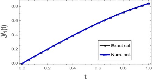
Figure 2. Comparing the numerical solution of ${\mathcal{Y}}_2\left(t\right)$ to test problem 1 with the exact solution.

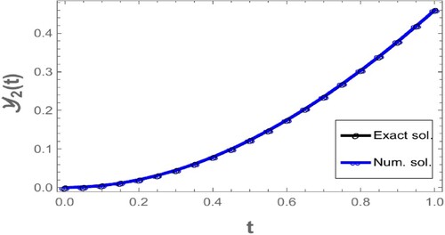
Table 1. Comparison between the exact and numerical solutions of test problem 1.

$t_i$	Numerical sol. of ${\mathcal{Y}}_1$	Exact solution of ${\mathcal{Y}}_1$	Absolute error of ${\mathcal{Y}}_1$	Numerical sol. of ${\mathcal{Y}}_2$	Exact solution of ${\mathcal{Y}}_2$	Absolute error of ${\mathcal{Y}}_2$
0.1	0.099792	0.099833	$4.11154\times {10}^{-5}$	0.005326	0.004996	$3.29772\times {10}^{-4}$
0.2	0.198538	0.198669	$1.31767\times {10}^{-4}$	0.020392	0.019934	$4.58849\times {10}^{-4}$
0.3	0.295265	0.295520	$2.54972\times {10}^{-4}$	0.045204	0.044664	$5.40578\times {10}^{-4}$
0.4	0.389015	0.389418	$4.02949\times {10}^{-4}$	0.079536	0.078939	$5.97302\times {10}^{-4}$
0.5	0.478855	0.479426	$5.70571\times {10}^{-4}$	0.123054	0.122417	$6.36325\times {10}^{-4}$
0.6	0.563888	0.564642	$7.54212\times {10}^{-4}$	0.175325	0.174664	$6.60446\times {10}^{-4}$
0.7	0.643266	0.644218	$9.51876\times {10}^{-4}$	0.235828	0.235158	$6.69828\times {10}^{-4}$
0.8	0.716192	0.717356	$1.16417\times {10}^{-4}$	0.303955	0.303293	$6.61737\times {10}^{-4}$
0.9	0.781931	0.783327	$1.39618\times {10}^{-3}$	0.379019	0.378390	$6.29112\times {10}^{-4}$

Test problem 2

Consider the following fractional q integro differential equation: (23) $\begin{array}{rl}& {\mathcal{D}}^{0.6}\left[{\mathcal{Y}}_1\right(t)-g_1(t,{\mathcal{Y}}_1(t+\varsigma ),{\mathcal{Y}}_2(t+\varsigma )\left)\right]\\ & =0.00993671t^{6/5}-0.00565335t^{11/5}\\ & -0.000778202t^{16/5}+0.000344551t^{21/5}\\ & +0.000203336t^{26/5}+0.000246612t^{31/5}\\ & -0.0000201867t^{36/5}+0.0000166928t^{41/5}\\ & -1.44133\times {10}^{-6}{t}^{46/5}+4.69655\times {10}^{-7}{t}^{51/5}\\ & -3.23018\times {10}^{-8}{t}^{56/5}+5.91518\times {10}^{-9}{t}^{61/5}\\ & +0.000648788t^{6.4}+0.0224221t^{4.4}\\ & +0.323329t^{2.4}-0.0145268t^{1.4}\\ & +1.11689t^{0.4}-0.018394e^t+0.05\\ & +\frac{1}{20}{e}^{t-1}{\mathcal{Y}}_1(t-1)+\frac{1}{20}{e}^{t-1}{\mathcal{Y}}_2(t-1)\\ & +\frac{1}{20}{I}_{0.4}^{\frac{6}{5}}{e}^{t-1}{\mathcal{Y}}_2\left(t-1\right),t\in [0,1],\\ & {\mathcal{D}}^{0.2}\left[{\mathcal{Y}}_2\right(t)-g_2(t,{\mathcal{Y}}_1(t+\varsigma ),{\mathcal{Y}}_2(t+\varsigma )\left)\right]\\ & =0.0172897t^{8/7}-0.00266982t^{15/7}\\ & -0.00176772t^{22/7}-0.000879239t^{29/7}\\ & -0.000491411t^{36/7}+0.0000132163t^{43/7}\\ & -0.0000603157t^{50/7}+5.4118\times {10}^{-6}{t}^{57/7}\\ & -2.5071\times {10}^{-6}{t}^{64/7}+1.8789\times {10}^{-7}{t}^{71/7}\\ & -4.2747\times {10}^{-8}{t}^{78/7}-0.0000379651t^{7.8}\\ & -0.00201367t^{5.8}-0.0560605t^{3.8}\\ & +0.00205292t^{2.8}-0.599705t^{1.8}\\ & -0.0138709t^{0.8}-0.0147152e^t+0.04\\ & +\frac{1}{25}{e}^{t-1}{\mathcal{Y}}_1(t-1)+\frac{1}{25}{e}^{t-1}{\mathcal{Y}}_2(t-1)\\ & +\frac{1}{25}{I}_{0.3}^{\frac{8}{7}}{e}^{t-1}{\mathcal{Y}}_1\left(t-1\right),t\in [0,1],\\ & {\mathcal{Y}}_1\left(t\right)=t+\frac{t^3}{6},{\mathcal{Y}}_2\left(t\right)=-\frac{t^2}{2}-\frac{t^4}{24},t\in [-1,0].\end{array}$(23) where $g_1(t,{\mathcal{Y}}_1(t+\varsigma ),{\mathcal{Y}}_2(t+\varsigma \left)\right)=2+\frac{1}{15}{e}^{t-1}{\mathcal{Y}}_1(t-1),g_2(t,{\mathcal{Y}}_1(t+\varsigma ),{\mathcal{Y}}_2(t+\varsigma \left)\right)=5+\frac{1}{18}{e}^{t-1}{\mathcal{Y}}_2(t-1).$ The exact solutions to this issue are ${\mathcal{Y}}_1\left(t\right)=\sinh \left(t\right),{\mathcal{Y}}_2\left(t\right)=1-\cosh \left(t\right).$ Suppose θ is a positive real constant and $\begin{array}{rl}{\mathcal{B}}_{\theta }& =\{{\mathcal{Y}}_i\in (C(-\mathrm{\infty },0],\mathbb{R}):\underset{\varsigma \to -\mathrm{\infty }}{lim}{e}^{\mathrm{\theta \varsigma }}{\mathcal{Y}}_i(\varsigma )\\ & \text{exist in}\mathbb{R},i=1,2\},\end{array}$with the norm $\begin{array}{rl}\Vert {\mathcal{Y}}_i{\Vert }_{{\mathcal{B}}_{\theta }}& =\{sup{e}^{\mathrm{\theta \varsigma }}|{\mathcal{Y}}_i(\varsigma )|,i=1,2,\varsigma \in (-\mathrm{\infty },0\left]\right\}.\end{array}$Let ${\mathcal{Y}}_i:(-\mathrm{\infty },d]\to \mathbb{R}$ be such that ${\mathcal{Y}}_{i,0}\in {\mathcal{B}}_{\theta },i=1,2$. Then $\begin{array}{rl}\underset{\varsigma \to -\mathrm{\infty }}{lim}{e}^{\mathrm{\theta \varsigma }}{\mathcal{Y}}_i(t+\varsigma )& =\underset{\varsigma \to -\mathrm{\infty }}{lim}{e}^{\theta (\varsigma -t)}{\mathcal{Y}}_i\left(\varsigma \right)\\ & =e^{-\theta t}\underset{\varsigma \to -\mathrm{\infty }}{lim}{e}^{\mathrm{\theta \varsigma }}{\mathcal{Y}}_i\left(\varsigma \right)<\mathrm{\infty }.\end{array}$Hence ${\mathcal{Y}}_i(t+\varsigma )\in {\mathcal{B}}_{\theta }$.

Finally, we demonstrate $\begin{array}{r}\Vert \left({\mathcal{Y}}_i\right(t+\varsigma ){\Vert }_{{\mathcal{B}}_{\theta }}\le {\kappa }_1(t\left)\underset{0\le \mathfrak{s}\le t}{sup}|{\mathcal{Y}}_1\right(\mathfrak{s})|+{\mu }_1(t)\Vert {\mathcal{Y}}_{1,0}{\Vert }_{{\mathcal{B}}_{\theta }},\end{array}$where ${\mathcal{K}}_1={\mathcal{M}}_1={\mathcal{K}}_2={\mathcal{M}}_2=1$, $\varrho =1.$ If $t+\varsigma \le 0,$ we get $\begin{array}{r}|{\mathcal{Y}}_i(t+\varsigma )|\le \underset{-\mathrm{\infty }<\mathfrak{s}\le 0}{sup}|{\mathcal{Y}}_i\left(\mathfrak{s}\right)|.\end{array}$For $t+\varsigma ⩾0,$ we get $\begin{array}{r}|{\mathcal{Y}}_i(t+\varsigma )|\le \underset{0<\mathfrak{s}\le t}{sup}|{\mathcal{Y}}_i\left(\mathfrak{s}\right)|.\end{array}$Thus for all $t+\varsigma \in (-\mathrm{\infty },d],$ we obtain $\begin{array}{r}|{\mathcal{Y}}_i(t+\varsigma )|\le \underset{-\mathrm{\infty }<\mathfrak{s}\le 0}{sup}|{\mathcal{Y}}_i\left(\mathfrak{s}\right)|+\underset{0<\mathfrak{s}\le d}{sup}|{\mathcal{Y}}_i\left(\mathfrak{s}\right)|.\end{array}$Therefore, $\begin{array}{r}\Vert \left({\mathcal{Y}}_i\right(t+\varsigma ){\Vert }_{{\mathcal{B}}_{\theta }}\le \Vert {\mathcal{Y}}_{i,0}{\Vert }_{{\mathcal{B}}_{\theta }}+\underset{0<\mathfrak{s}\le d}{sup}|{\mathcal{Y}}_i(\mathfrak{s})|.\end{array}$As a result, ${\mathcal{B}}_{\theta }$ is a phase space. We set $\begin{array}{rl}& {\mathcal{Z}}_1(t,{\mathcal{Y}}_1(t+\varsigma ),{\mathcal{Y}}_2(t+\varsigma ),I_{q_1}^{{\xi }_1}{\mathcal{Y}}_1(t+\varsigma ),I_{q_2}^{{\xi }_2}{\mathcal{Y}}_2(t+\varsigma \left)\right)\\ & =f_1\left(t\right)+\frac{1}{20}{e}^{t-1}{\mathcal{Y}}_1(t-1)+\frac{1}{20}{e}^{t-1}{\mathcal{Y}}_2(t-1)\\ & +\frac{1}{20}{I}_{0.4}^{\frac{6}{5}}{e}^{t-1}{\mathcal{Y}}_2(t-1)),\\ & {\mathcal{Z}}_2(t,{\mathcal{Y}}_1(t+\varsigma ),{\mathcal{Y}}_2(t+\varsigma ),I_{q_1}^{{\xi }_1}{\mathcal{Y}}_1(t+\varsigma ),I_{q_2}^{{\xi }_2}{\mathcal{Y}}_2(t+\varsigma \left)\right)\\ & =f_2\left(t\right)+\frac{1}{25}{e}^{t-1}{\mathcal{Y}}_1(t-1)+\frac{1}{25}{e}^{t-1}{\mathcal{Y}}_2(t-1)\\ & +\frac{1}{25}{I}_{0.3}^{\frac{8}{7}}{e}^{t-1}{\mathcal{Y}}_1(t-1),\end{array}$where $\begin{array}{rl}{f}_1\left(t\right)& =0.00993671t^{6/5}-0.00565335t^{11/5}\\ & -0.000778202t^{16/5}+0.000344551t^{21/5}\\ & +0.000203336t^{26/5}+0.000246612t^{31/5}\\ & -0.0000201867t^{36/5}+0.0000166928t^{41/5}\\ & -1.44133\times {10}^{-6}{t}^{46/5}+4.69655\times {10}^{-7}{t}^{51/5}\\ & -3.23018\times {10}^{-8}{t}^{56/5}+5.91518\times {10}^{-9}{t}^{61/5}\\ & +0.000648788t^{6.4}+0.0224221t^{4.4}\\ & +0.323329t^{2.4}-0.0145268t^{1.4}\\ & +1.11689t^{0.4}-0.018394e^t+0.05,\\ f_2\left(t\right)& =0.0172897t^{8/7}-0.00266982t^{15/7}\\ & -0.00176772t^{22/7}-0.000879239t^{29/7}\\ & -0.000491411t^{36/7}+0.0000132163t^{43/7}\\ & -0.0000603157t^{50/7}+5.4118\times {10}^{-6}{t}^{57/7}\\ & -2.5071\times {10}^{-6}{t}^{64/7}+1.8789\times {10}^{-7}{t}^{71/7}\\ & -4.2747\times {10}^{-8}{t}^{78/7}-0.0000379651t^{7.8}\\ & -0.00201367t^{5.8}-0.0560605t^{3.8}\\ & +0.00205292t^{2.8}-0.599705t^{1.8}\\ & -0.0138709t^{0.8}-0.0147152e^t+\mathrm{0.04.}\end{array}$As a result, we now have $\begin{array}{rl}& |{\mathcal{Z}}_1(t,{\mathcal{Y}}_1(t+\varsigma ),{\mathcal{Y}}_2(t+\varsigma ),I_{q_1}^{{\xi }_1}{\mathcal{Y}}_1(t+\varsigma ),I_{q_2}^{{\xi }_2}{\mathcal{Y}}_2(t+\varsigma \left)\right)|\\ & \le f_1\left(t\right)+\frac{1}{20}|e^{t-1}{\mathcal{Y}}_1(t-1)|+\frac{1}{20}|e^{t-1}{\mathcal{Y}}_2(t-1)|\\ & +\frac{1}{20}{I}_{0.4}^{\frac{6}{5}}|e^{t-1}{\mathcal{Y}}_2(t-1)|\\ & \le f_1\left(t\right)+\frac{1}{20}\Vert {\mathcal{Y}}_1(t-1){\Vert }_{{\mathcal{B}}_{\theta }}+\frac{1}{20}\Vert {\mathcal{Y}}_2(t-1){\Vert }_{{\mathcal{B}}_{\theta }}\\ & +\frac{1}{20}{I}_{0.4}^{\frac{6}{5}}\Vert {\mathcal{Y}}_2\left(t-1\right){\Vert }_{{\mathcal{B}}_{\theta }},\\ & |{\mathcal{Z}}_2(t,{\mathcal{Y}}_1(t+\varsigma ),{\mathcal{Y}}_2(t+\varsigma ),I_{q_1}^{{\xi }_1}{\mathcal{Y}}_1(t+\varsigma ),I_{q_2}^{{\xi }_2}{\mathcal{Y}}_2(t+\varsigma \left)\right)|\\ & \le f_2\left(t\right)+\frac{1}{25}|e^{t-1}{\mathcal{Y}}_1(t-1)|+\frac{1}{25}|e^{t-1}{\mathcal{Y}}_2(t-1)|\\ & +\frac{1}{25}{I}_{0.3}^{\frac{8}{7}}|e^{t-1}{\mathcal{Y}}_1(t-1)|\\ & \le f_2\left(t\right)+\frac{1}{25}\Vert {\mathcal{Y}}_1(t-1){\Vert }_{{\mathcal{B}}_{\theta }}+\frac{1}{25}\Vert {\mathcal{Y}}_2(t-1){\Vert }_{{\mathcal{B}}_{\theta }}\\ & +\frac{1}{25}{I}_{0.3}^{\frac{8}{7}}\Vert {\mathcal{Y}}_1(t-1){\Vert }_{{\mathcal{B}}_{\theta }}.\end{array}$Also, $\begin{array}{rl}& |g_1(t,{\mathcal{Y}}_1(t+\varsigma ),{\mathcal{Y}}_2(t+\varsigma \left)\right)|\le 2+\frac{1}{15}|e^{t+\varsigma }{\mathcal{Y}}_1(t+\varsigma )|\\ & \le 2+\frac{1}{15}\Vert {\mathcal{Y}}_1(t-1){\Vert }_{{\mathcal{B}}_{\theta }},\\ & |g_2(t,{\mathcal{Y}}_1(t+\varsigma ),{\mathcal{Y}}_2(t+\varsigma \left)\right)|\le 5+\frac{1}{18}|e^{t-1}{\mathcal{Y}}_2(t-1)|\\ & \le 5+\frac{1}{18}\Vert {\mathcal{Y}}_2(t-1){\Vert }_{{\mathcal{B}}_{\theta }}.\end{array}$Also, we have $\begin{array}{rl}{\varphi }_1& =(l_1{\mathcal{K}}_1+l_2{\mathcal{K}}_1+\frac{d^{{\alpha }_1}{\text{β}}_1{\mathcal{K}}_1}{\mathrm{\Gamma }({\alpha }_1+1)}+\frac{d^{{\alpha }_2}{\text{β}}_2{\mathcal{K}}_1}{\mathrm{\Gamma }({\alpha }_2+1)}\\ & +\frac{{\text{β}}_1{\mathcal{K}}_1{d}^{{\alpha }_1+{\xi }_1}\mathrm{\Gamma }(1+{\xi }_1)}{\mathrm{\Gamma }(1+{\alpha }_1+{\xi }_1){\mathrm{\Gamma }}_{q_1}({\xi }_1+1)}\\ & +\frac{{\text{β}}_2{\mathcal{K}}_1{d}^{{\alpha }_2+{\xi }_1}\mathrm{\Gamma }(1+{\xi }_1)}{\mathrm{\Gamma }(1+{\alpha }_2+{\xi }_1){\mathrm{\Gamma }}_{q_1}({\xi }_1+1)})\\ & =\frac{1}{15}+\frac{1}{18}+\frac{1}{20\mathrm{\Gamma }(0.6+1)}+\frac{1}{25\mathrm{\Gamma }(0.2+1)}\\ & +\frac{\mathrm{\Gamma }(\frac{6}{5}+1)}{20{\mathrm{\Gamma }}_{0.4}(\frac{6}{5}+1)\mathrm{\Gamma }(1+0.6+\frac{6}{5})}\\ & +\frac{\mathrm{\Gamma }(\frac{6}{5}+1)}{25{\mathrm{\Gamma }}_{0.4}(\frac{6}{5}+1)\mathrm{\Gamma }(1+0.2+\frac{6}{5})}\\ & =0.286616\le 1,\\ {\varphi }_2& =(l_1{\mathcal{K}}_2+l_2{\mathcal{K}}_2+\frac{d^{{\alpha }_1}{\text{β}}_1{\mathcal{K}}_2}{\mathrm{\Gamma }({\alpha }_1+1)}+\frac{d^{{\alpha }_2}{\text{β}}_2{\mathcal{K}}_2}{\mathrm{\Gamma }({\alpha }_2+1)}\\ & +\frac{{\text{β}}_1{\mathcal{K}}_2{d}^{{\alpha }_1+{\xi }_2}\mathrm{\Gamma }(1+{\xi }_2)}{\mathrm{\Gamma }(1+{\alpha }_1+{\xi }_2){\mathrm{\Gamma }}_{q_2}({\xi }_2+1)}\\ & +\frac{{\text{β}}_2{\mathcal{K}}_2{d}^{{\alpha }_2+{\xi }_2}\mathrm{\Gamma }(1+{\xi }_2)}{\mathrm{\Gamma }(1+{\alpha }_2+{\xi }_2){\mathrm{\Gamma }}_{q_2}({\xi }_2+1)})\frac{1}{15}+\frac{1}{18}\\ & +\frac{1}{20\mathrm{\Gamma }(0.6+1)}+\frac{1}{25\mathrm{\Gamma }(0.2+1)}\\ & +\frac{\mathrm{\Gamma }(\frac{8}{7}+1)}{20\mathrm{\Gamma }(1+0.6+\frac{8}{7}){\mathrm{\Gamma }}_{0.3}(\frac{8}{7}+1)}\\ & +\frac{\mathrm{\Gamma }(\frac{8}{7}+1)}{25\mathrm{\Gamma }(1+0.2+\frac{8}{7}){\mathrm{\Gamma }}_{0.3}(\frac{8}{7}+1)}\\ & =0.288888\le 1.\end{array}$where ${\alpha }_1=0.6,{\alpha }_2=0.2,{\text{β}}_1=\frac{1}{20},{\text{β}}_2=\frac{1}{25},l_1=\frac{1}{15},l_2=\frac{1}{18},d=1,{\xi }_1=\frac{6}{5},{\xi }_2=\frac{8}{7},q_1=0.4,q_2=0.3$.

As a result, the given issue has a unique solution. This problem can now be solved numerically, we can observe all the numerical results in Table 2, Figures 3 and 4:

Figure 3. Comparing the numerical solution of ${\mathcal{Y}}_1\left(t\right)$ to test problem 2 with the exact solution.

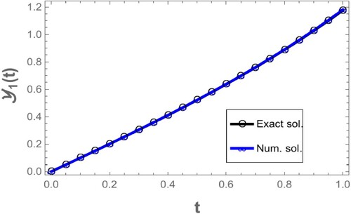
Figure 4. Comparing the numerical solution of ${\mathcal{Y}}_2\left(t\right)$ to test problem 2 with the exact solution.

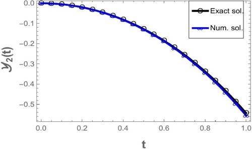
Table 2. Comparison between the exact and numerical solutions of test problem 2.

$t_i$	Numerical sol. of ${\mathcal{Y}}_1$	Exact solution of ${\mathcal{Y}}_1$	Absolute error of ${\mathcal{Y}}_1$	Numerical sol. of ${\mathcal{Y}}_2$	Exact solution of ${\mathcal{Y}}_2$	Absolute error of ${\mathcal{Y}}_2$
0.1	0.100198	0.100167	$3.13299\times {10}^{-5}$	−0.00524	−0.00500	$2.32208\times {10}^{-4}$
0.2	0.201458	0.201336	$1.21498\times {10}^{-4}$	−0.02051	−0.02007	$4.41656\times {10}^{-4}$
0.3	0.304769	0.304520	$2.49036\times {10}^{-4}$	−0.04612	−0.04534	$7.83753\times {10}^{-4}$
0.4	0.411170	0.410752	$4.17723\times {10}^{-4}$	−0.08239	−0.08107	$1.31574\times {10}^{-3}$
0.5	0.521745	0.521095	$6.49993\times {10}^{-4}$	−0.12972	−0.12763	$2.09102\times {10}^{-3}$
0.6	0.637641	0.636654	$9.87615\times {10}^{-4}$	−0.18863	−0.18547	$3.16877\times {10}^{-3}$
0.7	0.760078	0.758584	$1.49431\times {10}^{-3}$	−0.25979	−0.25517	$4.61799\times {10}^{-3}$
0.8	0.890365	0.888106	$2.25949\times {10}^{-3}$	−0.34396	−0.33744	$6.52055\times {10}^{-3}$
0.9	1.029919	1.026516	$3.40298\times {10}^{-3}$	−0.44206	−0.43309	$8.97432\times {10}^{-3}$

6. Conclusion

The coupled system of fractional q integro differential equations with infinite delay has been the subject of discussion regarding its existence and distinctness of solutions. The combination of the trapezoidal method and the finite difference method is used to arrive at the problem's numerical solution. Finally, two cases are numerically solved and compared with the exact solutions to show the efficacy of the strategy adopted. The methods used were accurate and reliable, as evidenced by the excellent correlation found between the numerical and exact solutions. The results of this study have important ramifications since they open up new avenues for research into fractional q-integro-differential equations with infinite delays. Researchers interested in this fascinating topic can benefit greatly from the tools and methodologies provided in this study. We have made significant progress in solving the riddles these intricate equations hold by connecting theoretical analysis and real-world computation. We have made significant contributions to the understanding of the existence, uniqueness, and numerical approximation of solutions for fractional q-integro-differential equations with infinite delays as a result of our persistent quest of knowledge. The significance of this study goes beyond mathematics since it advances our comprehension of real-world phenomena and promotes scientific advancement. Indeed, the work done here will lay a strong basis for future discoveries as scientists continue to delve into the complexities of fractional q-integro-differential equations. Through embracing the combination of theory and computation, we set out on a research trajectory that is extremely promising in terms of theoretical advances as well as real-world applications.

Ethics approval and consent to participate

The author confirm that all the results they obtained are new and there is no conflict of interest with anyone.

Consent for publication

The paper has one author who agrees to publish.

Authors' Contribution

If we look at the contribution of each author in this paper, we will find that each of them participated in the work from beginning to end in equal measure.

Acknowledgements

The authors extend their appreciation to Taif University, Saudi Arabia, for supporting this work through project number (TU-DSPP-2024-73).

Disclosure statement

No potential conflict of interest was reported by the author(s).

Availability of data and materials

Data sharing is not applicable to this article as no data sets were generated or analyzed during the current study.

Additional information

Funding

The authors extend their appreciation to Taif University, Saudi Arabia, for supporting this work through project number (TU-DSPP-2024-73).

References

- Tunç O, Tunç C, Petrusel G, et al. On the Ulam stabilities of nonlinear integral equations and integro-differential equations. Math Methods Appl Sci. 2024;47:4014–4028. doi: 10.1002/mma.v47.6
- Tunç O, Tunç C. Ulam stabilities of nonlinear iterative integro-differential equations. Rev Real Acad Cienc Exactas Fis Nat Ser A-Mat. 2023;117:118. doi: 10.1007/s13398-023-01450-6
- Tunç O, Tunç C. On Ulam stabilities of iterative fredholm and Volterra integral equations with multiple time-varying delays. Rev Real Acad Cienc Exactas Fis Nat Ser A-Mat. 2024;2024:20.
- Mahto L, Abbas S, Favini A. Analysis of Caputo impulsive fractional order differential equations with applications. Int J Differ Equations. 2013;2013:11. doi: 10.1155/2013/704547
- Abbas S. Pseudo almost automorphic solutions of fractional order neutral differential equation. Semigroup Forum. 2010;81:393–404. doi: 10.1007/s00233-010-9227-0
- Abbas S. Existence of solutions to fractional order ordinary and delay differential equations and applications. Electronic J Differ Equations. 2011;2011:1–11.
- Benchohra M, Henderson J, Ntouyas SK, et al. Existence results for fractional order functional differential equations with infinite delay. J Math Anal Appl. 2008;338:1340–1350. doi: 10.1016/j.jmaa.2007.06.021
- Babakhani A, Baleanu D, Agarwal RP. The existence and uniqueness of solutions for a class of nonlinear fractional differential equations with infinite delay. Abstract Appl Anal. 2013;2013:8. doi: 10.1155/2013/592964
- Liu J, Zhao K. Existence of mild solution for a class of coupled systems of neutral fractional integro-differential equations with infinite delay in Banach space. Adv Differ Equation. 2019;2019:15. doi: 10.1186/s13662-019-1951-5
- Ravichandran C, Baleanu D. Existence results for fractional neutral functional integro-differential evolution equations with infinite delay in Banach spaces. Adv Differ Equations. 2013;2013:12. doi: 10.1186/1687-1847-2013-12
- Hameed AK, Mustafa MM. Numerical solution of linear fractional differential equation with delay through finite difference method. Iraqi J Sci. 2022;63:1232–1239. doi: 10.24996/ijs.2022.63.3.28
- Ibrahim AA, Zaghrout AAS, Raslan KR, et al. On the analytical and numerical study for nonlinear Fredholm integro-differential equations. Appl Math Inf Sci. 2020;14:921–929. doi: 10.18576/amis
- Raslan KR, Ali KK, Ahmed RG, et al. Study of nonlocal boundary value problem for the Fredholm–Volterra integro-differential equation. Hindawi J Function Spaces. 2022;2022:16.
- Ibrahim AA, Zaghrout AAS, Raslan KR, et al. On the analytical and numerical study for fractional q-integrodifferential equations. Boundary Value Probl. 2022;2022:15. doi: 10.1186/s13661-022-01601-5
- Ibrahim AA, Zaghrout AAS, Raslan KR, et al. On study nonlocal integro differetial equation involving the Caputo-Fabrizio fractional derivative and q-integral of the riemann liouville type. Appl Math Inf Sci. 2022;16:983–993. doi: 10.18576/amis
- Ali KK, Raslan KR, Ibrahim AA, et al. On study the fractional Caputo-Fabrizio integro differential equation including the fractional q-integral of the Riemann-Liouville type. AIMS Math. 2023;8:18206–18222. doi: 10.3934/math.2023925
- Ibrahim AA, Zaghrout AAS, Raslan KR, et al. On study of the coupled system of nonlocal fractional q-integro-differential equations. Int J Modeling, Simulation, Scientific Comput. 2022;14:26.
- Ali KK, Raslan KR, Ibrahim AA, et al. The nonlocal coupled system of Caputo–Fabrizio fractional q-integro differential equation. Math Methods Appl Sci. 2023;2023:17.
- Hale J, Kato J. Phase space for retarded equations with infinite delay. Funkcial Ekvac. 1978;21:11–41.
- Hino Y, Murakami S, Naito T. Functional differential equations with infinite delay. Berlin: Springer-Verlag; 1991. (Lecture Notes in Mathematics; vol. 1473).
- Kilbas A, Srivastava MH, Trujillo JJ. Theory and application of fractional differential equations. 2006. (North Holland Mathematics Studies; vol. 204).
- Ahmad B, Nieto JJ, Alsaedi A, et al. Existence of solutions for nonlinear fractional q-difference integral equations with two fractional orders and nonlocal four-point boundary conditions. J Franklin Inst. 2014;351:2890–2909. doi: 10.1016/j.jfranklin.2014.01.020
- Annaby MH, Mansour ZS. q-fractional calculus and equations. London: Springer; 2012.
- Smart DR. Fixed point theorems. Cambridge: Cambridge University Press; 1974.