Understanding the dynamical mechanism of year-to-year incremental prediction by nonlinear time series prediction theory

Abstract

Previous studies have shown that year-to-year incremental prediction (YIP) can obtain considerable skill in seasonal forecasts. This study analyzes the mathematical definition of YIP and derives its formula in the nonlinear time series prediction (NP) method. It is shown that the two methods are equivalent when the prediction time series is embedded in one-dimensional phase space. Compared to previous NP models, the new one introduces multiple external forcings in the form of year-to-year increments. The year-to-year increments have physical meaning, which is better than the NP model with empirically chosen parameters. The summer rainfall over the middle to lower reaches of the Yangtze River is analyzed to examine the prediction skill of the NP models. Results show that the NP model with year-to-year increments can reach a similar skill as the YIP model. When the embedded number of dimensions is increased to two, more accurate prediction can be obtained. Besides similar results, the NP method has more dynamical meaning, as it is based on the classical reconstruction theory. Moreover, by choosing different embedded dimensions, the NP model can reconstruct the dynamical curve into phase space with more than one dimension, which is an advantage of the NP model. The present study suggests that YIP has a robust dynamical foundation, besides its physical mechanism, and the modified NP model has the potential to increase the operational skill in short-term climate prediction.

摘要

基于年际增量预测（YIP）方法的数学原理，推导得出新的非线性时间序列预测(NP)方法，并从理论上证明了两种预测方法在一定条件下的等效性。以长江中下游地区的夏季降水为例，新的NP方法在使用年际增量作为强迫项时，可以取得与YIP相当的预测效果。而且，通过调整重构维数等参数，能够将预测模型重构于高于一维的相空间中，进而可获得更好的预测效果。研究发现YIP方法除了有物理基础外，还有隐含的动力基础，新NP模型有助于提高短期气候预测的水平。

Keywords:

• Year-to-year incremental prediction
• nonlinear time series prediction
• precipitation
• Yangtze River
• seasonal prediction

关键词:

• 年际增量
• 非线性时间序列
• 降水
• 季节预测

1. Introduction

Short-term climate prediction is a hot but challenging scientific topic in current climate research. According to previous studies, the methods frequently used in short-term climate prediction include: the statistical approach, the hybrid statistical and dynamical approach, the numerical model approach, and the nonlinear time series prediction approach (hereafter NP). The latter is based on the phase-space reconstruction theorem (Casdagli 1989), which implicitly requires a stationary system. However, weather and climate systems are influenced by perturbations of driving forces; in other words, the atmosphere is essentially nonstationary in dynamic terms. Previous studies have indicated that the stationarity of atmospheric processes is changeable. For instance, Tsonis (1996) found that fluctuations around the global mean precipitation amount have increased significantly, which means that global precipitation was a nonstationary process over the past century. The cause of nonstationarity is the change in driving forces with time (Manuca and Savit 1996). This led Wang et al. (2011) to develop a new prediction model with such driving forces, which can improve the accuracy of prediction effectively when applied to the time series of a single climate variable.

However, most time series from the real world, especially those of processes typically related to climate, are too short. When we apply the NP method to such short time series, the model sometimes encounters a data ‘bottleneck’. Researchers have thus proposed the ‘spatiotemporal series’ method, which attempts to utilize the information at different spatial positions to remedy the insufficiency in the length of the time series. For example, with a spatiotemporal artificial neural network system, Yang, Zhou, and Bian (2000) carried out a regional prediction experiment regarding the distribution of atmospheric ozone over China, and the accuracy of the prediction was beyond 43%. In addition, based on the spatiotemporal series method, Chen et al. (2003) improved the extended-range (monthly) dynamical prediction of the pentad zonal mean height and revealed that spatiotemporal series can effectively improve the ergodicity of single-variable time series. Wang, Yang, and Lü (2004) introduced the idea of spatiotemporal series to enhance the original NP method and, through the example of 500 hPa height over the Northern Hemisphere, found that it is valuable to apply this technique to regional climate prediction.

In short-term climate prediction, the predictands are traditional climate variable anomalies (Wang et al. 2012). As most regions in East Asia vary in connection to the tropospheric biennial oscillation (TBO), it may be easy to capture the interannual change if the prediction method takes the TBO into consideration. However, decadal change in the climate mean may lead to uncertainty in the prediction. To deal with this issue, Fan, Wang, and Choi (2008) proposed a new prediction scheme in their study of summer rainfall over the middle to lower reaches of the Yangtze River, named the year-to-year incremental prediction (YIP) method. Hereafter, we use YR to stand for the summer rainfall in this region. In this approach, the first stage is to predict the year-to-year precipitation increments, and the precipitation and precipitation rate anomalies are computed. The average root-mean-square error (RMSE) of the fitting period is 20%, and 18% in the hindcast stage of YR. The prediction model captures the interannual variation of YR, and reproduces the ascending trend in 1984–1998 and the descending trend in 1998–2006, and thus raises the prediction skill of YR strikingly. This method has also been applied to the prediction of summer rainfall in North China (Fan, Lin, and Gao 2009), winter surface air temperature (Fan 2009) and summer temperature (Fan and Wang 2010) over Northeast China, typhoon frequency over the western North Pacific (Fan and Wang 2009), wintertime heavy snow activity in Northeast China (Fan and Tian 2013), and the North Atlantic Oscillation (Tian and Fan 2015), among other climatic features.

There have been many variants of YIP, but the fundamental method is that based on Fan, Wang, and Choi (2008). The benefit of YIP is that it involves physical mechanics, while the advantage of NP is that it has robust mathematical dynamical foundations. By combining YIP and NP, we may achieve a better understanding of YIP with respect to its dynamical mechanism. In addition, we can analyze its advantages and disadvantages, and then explore its potential for application to other seasonal events in short-term climate prediction.

2. Data and methods

Monthly precipitation data from 160 stations (1964–2006) in China provided by the China Meteorological Administration are used in this study. Following Chen and Zhao (2000), the mean precipitation of 17 stations during June–August over the middle to lower reaches of the Yangtze River (Nanjing, Hefei, Shanghai, Hangzhou, Anqing, Tunxi, Jiujiang, Hankou, Zhongxiang, Yueyang, Yichang, Changde, Ningbo, Quxian, Guixi, Nanchang, and Changsha) is selected to represent the summer rainfall over this region.

The present study employs monthly atmospheric variables from the NCEP–NCAR reanalysis data set, with a resolution of 2.5° × 2.5° (Kalnay et al. 1996).

2.1. The YIP method

The YR can be predicted on the basis of precursory factors using the YIP model (Fan, Wang, and Choi 2008).(1)

where ΔY stands for the year-to-year increments of YR, Δf is the year-to-year increments of the normalized indices (also known as DY — the difference of a variable between the current year and the preceding year), c_i is the fitting parameter, and the subscript in Δf represents the number of the predictor.

Each Δf is defined as(2)

where N is the number of years of historical data. The details of six factors can be found in Fan, Wang, and Choi (2008) (also introduced in Section 3.1 in the present paper).

2.2. The NP method with external forcing

The method of using a single-point nonlinear model with driving forces refers to the work of Wang et al. (2011) and Wang, Yang, and Zhou (2013). Assuming a non-stationary process with two series and , the former variable is the system state and the latter is the driving force. By selecting a proper parameter τ, we can embed them into a state space (also known as phase space) with m₁ + m₂ dimensions, and then obtain the state trajectory(3)

where m₁ and m₂ are the dimensions of and , respectively; and is the number of points in phase space. After reconstructing this trajectory, we can build a prediction model by means of the global approximation method (Casdagli 1989),(4)

where is an undetermined function, is the system state, is the driving force, and ɛ_i is the fitting residual. The condition to determine is to make the sum of the squared residuals reach its minimum,(5)

Here, φ is supposed to be a second-order polynomial at most.

The single-point prediction method can be expanded to the spatial time series prediction method, which not only includes the driving forces but also the information from the surrounding four neighboring points. The spatiotemporal series prediction model can be written as(6)

The embedding dimension of is m₁, and the forcings and are embedded in the m₂ dimension (in this study, we choose m₁ = m₂ = m).

2.3. Relationship between YIP and NP

Once the sample number N in YIP is large enough, we have and then(7)

where C is the expected value of , and ΔY = c₁Δf₁ + c₂Δf₂ + c₃Δf₃ + c₄Δf₄ + c₅Δf₅ + c₆Δf₆ is equivalent to(8)

Let , and we have(9)

This formula is analogue to the NP model (Equation (4(4) )). This implies that they have some corresponding relationship. Equation (4(4) ) only considers one forcing originally, but we can expand it to multiple forcings and one variable system by way of Equation (6(6) ):(10)

Here, ɛ_t is the fitting residual. The model only uses the value of one previous step during prediction, so it can be regarded as an NP model with m = 1 and τ = 1 to predict one step ahead. Therefore, we can conclude that YIP and NP are equivalent when linear fitting is applied and N is large enough.

From the theoretical analysis, YIP could be considered as a special case of NP, so the YIP method can be applied to nonlinear modeling. YIP emphasizes the effect of quasi-biennial signals; thus, this method has explicit physical meaning compared with the NP method.

3. Hindcast and result

To reveal the equivalence of YIP and NP, and compare their performance, we apply the two methods to the following rainfall prediction experiments.

3.1. Precipitation prediction of YIP

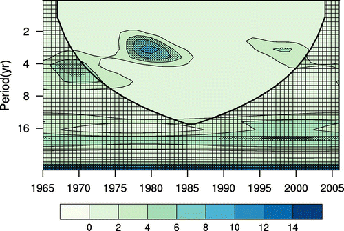
Figure 1 shows the wavelet analysis of YR. It illustrates that there is a strong 2–5-yr period of YR variations in the period 1965–2006, so we can amplify the anomaly signal of the rainfall via YIP.

Figure 1. The wavelet power spectrum of the summer mean precipitation in the middle to lower reaches of the Yangtze River during 1965–2006.

Notes: The dotted regions are greater than the 95% confidence level for a red noise process; cross-hatched regions show the ‘cone of influence’.

Fan, Wang, and Choi (2008) analyzed the correlation coefficients between the year-to-year increments of YR and the geopotential height field at 500 hPa in spring and found that the Urals high and East Asian trough have a great influence on YR. So they defined two indices: the spring Eurasian circulation index (EUI) and the spring East Asian circulation index (EAI). The EUI is the area-averaged geopotential height at 500 hPa over the region (60°–70°N, 30°–60°E), and the correlation coefficient between the year-to-year increments of YR and EUI is 0.41 during 1965–1996, reaching the 95% confidence level. The EAI is the area-averaged geopotential height at 500 hPa over the region (55°–60°N, 120°–150°E), and the correlation coefficient between the year-to-year increments of YR and the EAI is −0.44 during 1965–1996, reaching the 95% confidence level.

Figure 2 depicts the correlation coefficients between the year-to-year increments of YR and meridional wind shear between the 850 hPa and 200 hPa levels in March–May (MAM) (i.e. v850 minus v200). As is shown in Figure 2, there is negative correlation in the region of (20°S–10°N, 120°–140°E), which is the place for the interaction of the monsoon and ENSO. Next, we define an index for meridional wind shear around Indo-Australia (WSI) using the area-averaged meridional wind shear over the region (20°S–10°N, 120°–140°E). The correlation coefficient between the year-to-year increments of YR and the WSI is −0.33 during 1965–1996, reaching the 90% confidence level.

Figure 2. Correlation coefficients between the year-to-year increments of the summer rainfall over the middle to lower reaches of the Yangtze River and meridional wind shear between the 850 hPa and 200 hPa levels in March–May during 1965–1996.

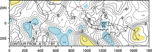
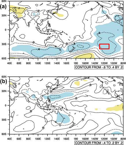
Figure 3(a) reveals the correlation coefficients between the year-to-year increments of YR and sea level pressure in December–February (DJF). According to Figure 3(a), there is a remarkable negative-correlation area in the South Pacific. Therefore, we define a South Pacific sea level pressure index (SPI) using the area-averaged sea level pressure over the region (40°–30°S, 130°–110°W). The correlation coefficient between the year-to-year increments of YR and the SPI is −0.49 during 1965–1996, reaching the 99% confidence level. Figure 3(b) shows the correlation coefficients between the year-to-year increments of the SPI in DJF and the sea level pressure in JJA. The result indicates that the SPI in winter is linked to the western Pacific subtropical high in summer.

Figure 3. (a) Correlation coefficients between the year-to-year increments of the summer rainfall over the middle to lower reaches of the Yangtze River and the sea level pressure in December–February (DJF) during 1965–1996. (b) Correlation coefficients between the year-to-year increments of the index for South Pacific sea level pressure in DJF and the sea level pressure in June–August (JJA) during 1965–1996.

When analyzing the correlation coefficients between the year-to-year increments of YR and vorticity at 850 hPa, obvious positive coefficients are found in the region (30°–35°N, 115°–120°E) from spring to summer. Thus, we consider the vorticity index (VOI), i.e. the 850-hPa vorticity averaged in the above region, as a factor in the prediction of YR year-to-year increments. The correlation coefficient between the year-to-year increments of YR and the VOI is 0.49 during 1965–1996, reaching the 99% confidence level.

Fan, Wang, and Choi (2008) considered the AAO (Antarctic Oscillation) index as well, but we find that the correlation coefficient of the year-to-year increments of YR and the AAO is relatively small. There is no significant difference in the prediction when we exclude the AAO index. Hence, we do not take the AAO index into account in this paper.

We build the YIP prediction model based on the year-to-year increments of five factors from 1965 to 1996 in order to predict the YR, and then conduct the hindcast in the following 10 years. The statistical forecast model of YR year-to-year increments through the multi-linear regression is(11)

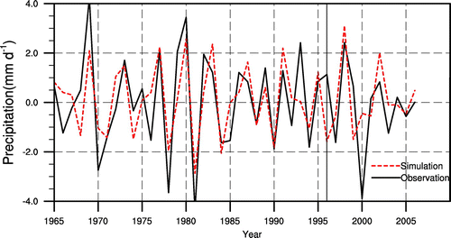
Figure 4 illustrates the simulated and observed year-to-year increments of YR from 1965 to 2006. It suggests that the simulated increments from the above five factors resemble the observations quite well. The correlation coefficient between the model result and observation is 0.74 in 1965–1996, and 0.56 in 1997–2006. There is an obvious biennial variation in the year-to-year increments of YR, which features alternately positive and negative anomalies in neighboring years. Most of the years with large positive and negative anomalies during the previous period from 1965 to 1996, such as in 1977, 1978, 1980, and 1981, are simulated by the model successfully. During the hindcast in 1997–2006, the model reproduces the years of extremely high YR increments, such as in 1998 and 2002. Relatively, for the year 2000, which has an extremely negative YR increment, the model does not behave well, but it still produces a negative increment.

Figure 4. Time series of observed (black solid line) and simulated (red dashed line) year-to-year increments of summer rainfall over the middle to lower reaches of the Yangtze River during 1965–2006.

3.2. Precipitation prediction of NP

When using the NP method to build the prediction model, we utilize the same five factors and the former 32-yr precipitation data to reconstruct the phase trajectory, and then conduct one-step prediction in the latter 10 years to examine the performance. In the model, we choose the embedded dimensions as m = 1 and m = 2, respectively, and the time delay parameter as τ = 1.

The NP results are consistent with the observed values (Figure 5). In the middle to lower reaches of the Yangtze River, NP can capture the upward trend at the end of the twentieth century, and the downward trend after 2000. For the years with a large amount of precipitation, the predicted values are similar to observed, such as in 1997 and 1983. For the years with a fairly small amount of precipitation, the prediction model also behaves well, such as in 1972 and 1981. Overall, the YIP and NP methods predict similar results.

Figure 5. Observed and predicted summer precipitation over the middle to lower reaches of the Yangtze River from 1965 to 2006.

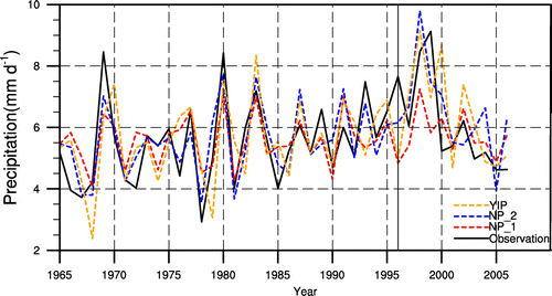
Though the correlation coefficient of the NP model (m = 1) in the building stage is smaller than that in YIP (Table 1), the correlation coefficient in the predicting stage is similar to YIP. We also apply the NP model with a higher number of embedded dimensions (m = 2) and find an increased correlation coefficient (Table 1).

Table 1. Correlation coefficients between the prediction and observation in different models.

	Correlation in the building stage	Correlation in the predicting stage
NP (m = 2)	0.819	0.706
NP (m = 1)	0.588	0.565
YIP	0.742	0.561

Notes: NP, nonlinear time series prediction method; m, number of embedded dimensions; YIP, year-to-year incremental prediction method.

To further evaluate the accuracy of precipitation prediction, we define two quantities: the percentage of relative error of prediction,(12)

And the average relative RMSE,(13)

Here, y is the simulated YR, y₀ is the observation, and is the multi-year average precipitation from 1965 to 1996.

Table 2 depicts the percentage errors of prediction from 1997 to 2006. Most of the precipitation errors are smaller than 30%, except in 1999 and 2000. This indicates that all three models are efficient in predicting YR. However, these models all still have large prediction errors in 1999 and 2000. Generally, the NP method may obtain similar results to the YIP method. When we compare the results of two cases of the NP method, the precipitation mean-square error is a little lower when the number of embedded dimensions is set to two rather than one. The mean-square errors (1997–2006) of the three models (YIP, NP (m = 1) and NP (m = 2)) are 26.62%, 22.71%, and 22.30%, respectively.

Table 2. Relative percentage error of prediction (%).

	YIP	NP (m = 1)	NP (m = 2)
1997	19.45	−11.39	11.25
1998	12.44	−22.01	24.13
1999	−38.94	−59.54	−29.87
2000	62.36	19.28	32.85
2001	−12.69	−1.74	2.22
2002	21.30	7.14	−14.18
2003	20.63	9.32	17.28
2004	−5.54	6.15	26.14
2005	1.86	4.66	−12.36
2006	8.56	20.55	30.85
	RMSE
	26.62	22.71	22.30

Notes: NP, nonlinear time series prediction method; m, number of embedded dimensions; YIP, year-to-year incremental prediction method.

4. Conclusion

The YIP method is based on the knowledge that the physical processes of the predictands and the climate variables have the characteristics of quasi-biennial variation. Therefore, we can use the preceding year’s observational information as much as possible to improve the prediction results. Previous research has revealed that the YIP approach may improve the forecast skill (Wang et al. 2012). We analyze the mathematical definition of YIP and obtain its corresponding formula in the NP method. It proves that they are equivalent when the prediction time series is embedded in one-dimensional phase space. This theoretical result suggests that YIP also has robust mathematical and dynamical foundations, besides its physical mechanism.

We demonstrate the NP model with multiple external driving forces. The model is different from previous NP models in its application of year-to-year increments (Δf) as forcing factors. Hence, the quasi-biennial signals with explicit physical meaning are included, which is better than the NP model with empirically chosen parameters. In a certain sense, the two models are equivalent. Nevertheless, the NP method has more dynamical meaning, as it is based on the classical reconstruction theory. By choosing different embedded dimensions, the NP model can reconstruct the dynamical curve into phase space with a higher number of dimensions than one. In addition, the fitting residual of NP can be set to second-order polynomial precision, which is more convenient than the original linear regression of YIP, indicating the superiority of the NP model over the YIP model. We also notice that YIP and NP have some differences when the sample number N is not big enough, and these differences can decrease with an increase in N. The numerical results suggest that these differences are acceptable in practical prediction experiments.

We select the YR to test the prediction skill of the NP models. Five predictors are introduced into the YIP and NP models. Results show that the NP model with year-to-year increments of former signals can obtain similar skill as the YIP model. When we increase the number of embedded dimensions to two, more accurate prediction can be obtained. These results indicate that the NP model has the potential to increase the operational skill in short-term climate prediction.

Disclosure statement

No potential conflict of interest was reported by the authors.

Funding

This work was supported by the National Natural Sciences Foundation of China [41375112], [41530426], [41575058]; the Key Technology Talent Program of the Chinese Academy of Sciences; the Public Science and Technology Research Funds Projects of Ocean [201505013].

Acknowledgments

Pengfei WANG acknowledges Prof. Geli WANG for providing the FORTRAN code of the nonlinear time series prediction.

References

- Casdagli, M. 1989. “Nonlinear Prediction of Chaotic Time Series.” Physica D: Nonlinear Phenomena 35 (3): 335–356. doi:10.1016/0167-2789(89)90074-2.
- Chen, B. M., L. R. Ji, P. C. Yang, D. M. Zhang, and G. L. Wang. 2003. “An Approach to Improving the Dynamical Extended-range (Monthly Prediction).” Chinese Science Bulletin 48 (7): 696–703. doi:10.1007/BF03325658.
- Chen, X. F., and Z. G. Zhao. 2000. “Climatic Analysis of Summer Precipitation.” In The Investigation of Flood Season Precipitation Prediction in China and its Application [in Chinese], 8–9. Beijing: Meteorological Press.
- Fan, K. 2009. “Predicting Winter Surface Air Temperature in Northeast China.” Atmospheric and Oceanic Science Letters 2 (1): 14–17. doi:10.1080/16742834.2009.11446770.
- Fan, K., M. J. Lin, and Y. Z. Gao. 2009. “Forecasting the Summer Rainfall in North China Using the Year-to-year Increment Approach.” Science in China Series D: Earth Sciences 52 (4): 532–539. doi:10.1007/s11430-009-0040-0.
- Fan, K., and B. Q. Tian. 2013. “Prediction of Wintertime Heavy Snow Activity in Northeast China.” Chinese Science Bulletin 58 (12): 1420–1426. doi:10.1007/s11434-012-5502-7.
- Fan, K., and H. J. Wang. 2009. “A New Approach to Forecasting Typhoon Frequency over the Western North Pacific.” Weather and forecasting 24 (4): 974–986. doi:10.1175/2009WAF2222194.1.
- Fan, K., and H. J. Wang. 2010. “Seasonal Prediction of Summer Temperature over Northeast China Using a Year-to-year Incremental Approach.” Acta Meteorologica Sinica 24 (3): 269–275.
- Fan, K., H. J. Wang, and Y.-J. Choi. 2008. “A Physically-based Statistical Forecast Model for the Middle-lower Reaches of the Yangtze River Valley Summer Rainfall.” Chinese Science Bulletin 53 (4): 602–609. doi:10.1007/s11434-008-0083-1.
- Kalnay, E., M. Kanamitsu, R. Kistler, W. Collins, D. Deaven, L. Gandin, M. Iredell, et al. 1996. “The NCEP/NCAR 40-year Reanalysis Project.” Bulletin of the American Meteorological Society 77: 437–470. doi:10.1175/1520-0477(1996)077<0437:TNYRP>2.0.CO;2.
- Manuca, R., and R. Savit. 1996. “Stationarity and Nonstationarity in Time Series Analysis.” Physica D: Nonlinear Phenomena 99 (2–3): 134–161. doi:10.1016/S0167-2789(96)00139-X.
- Tian, B., and K. Fan. 2015. “A Skillful Prediction Model for Winter NAO Based on Atlantic Sea Surface Temperature and Eurasian Snow Cover.” Weather and Forecasting 30 (1): 197–205. doi:10.1175/WAF-D-14-00100.1.
- Tsonis, A. 1996. “Widespread Increases in Low-frequency Variability of Precipitation over the Past Century.” Nature 382 (6593): 700–702. doi:10.1038/382700a0.
- Wang, H. J., K. Fan, X. M. Lang, J. Q. Sun, and L. J. Chen. 2012. The New Theory. Method and Technology for the Short-term Climate Prediction in China [in Chinese]. Beijing: Meteorological Press.
- Wang, G. L., P. C. Yang, J. Bian, and X. J. Zhou. 2011. “A Novel Approach in Predicting Non-stationary Time Series by Combining External Forces.” Chinese Science Bulletin 56 (z2): 3053–3056. doi:10.1007/s11434-011-4638-1.
- Wang, G. L., P. C. Yang, and D. R. Lü. 2004. “On Spatiotemporal Series Analysis and Its Application to Predict the Regional Short Term Climate Process.” Advances in Atmospheric Sciences 21 (2): 296–299. doi:10.1007/BF02915717.
- Wang, G. L., P. C. Yang, and X. J. Zhou. 2013. “Nonstationary Time Series Prediction by Incorporating External Forces.” Advances in Atmospheric Sciences 30 (6): 1601–1607. doi:10.1007/s00376-013-2134-z.
- Yang, P. C., X. J. Zhou, and J. C. Bian. 2000. “A Nonlinear Regional Prediction Experiment on a Short-range Climatic Process of the Atmospheric Ozone.” Journal of Geophysical Research Atmospheres 105 (D10): 12253–12258. doi:10.1029/2000JD900098.