New approach to incorporating the impacts of non-hydrostatic perturbations in atmospheric models

Abstract

How to properly consider the impacts of non-hydrostatic perturbations is one of the challenging issues in developing non-hydrostatic dynamics solvers (NHDSs) for high-resolution atmospheric models. To overcome the drawbacks of current approaches to tackling this issue, this study analyzed the differences between hydrostatic dynamics solvers (HDSs) and their non-hydrostatic counterparts. The analysis then motivated a flexible approach to adjusting existing hydrostatic atmospheric models, especially those adopted in climate simulations for the impacts of non-hydrostatic perturbations. In this approach, the impacts of non-hydrostatic perturbations, reflecting the differences between HDSs and NHDSs, were encapsulated into a single term in the vertical momentum equation for the atmosphere. At each time step, this term was estimated by a separate sub-model, and then it was used to adjust the dynamics of the atmosphere. The adjustment was optional, and could be turned on and off flexibly by utilizing different initial conditions. The approach was illustrated using the Weather Research and Forecasting (WRF) model as an example, and was preliminarily validated by running the 3D baroclinic-wave test case in the model. Results showed that the modified dynamics solver produced simulation results that were very close to those given by the standard NHDS in the WRF model, implying that the approach was basically effective in capturing the non-hydrostatic features of the atmosphere.

摘要

通过对静力和非静力模式动力框架进行对比分析，研究发现：非静力扰动主要影响大气的垂直运动，对于水平运动的影响相对而言较小，且其影响可通过一个控制其打开和关闭状态的开关性变量来予以表示。基于上述发现，提出了一套新的非静力扰动整合方案。该方案将复杂耗时的偏微分方程数值求解问题转化为基于历史数据的局部函数建模问题，且能够比较方便地应用于一般的静力模式动力框架当中，大大降低了非静力大气环流模式的研发难度和工作量。

Keywords:

• Hydrostatic
• non-hydrostatic
• dynamics solver
• WRF

关键词:

• 静力
• 非静力
• 动力框架
• WRF

1. Introduction

With the great advances achieved in computer technology, there is a trend in the atmospheric modeling community toward developing high-resolution non-hydrostatic atmospheric models for climate simulations (Hall 2013). Examples of efforts in this direction include the Non-hydrostatic Icosahedral Atmospheric Model (Satoh et al. 2008); Atmospheric Model, version 3 (Donner et al. 2010); and the in-progress PantaRhei project (Smolarkiewicz, Kühnlein, and Wedi 2014). One of the challenging problems encountered in developing these models is to incorporate the non-hydrostatic features of the atmosphere in an appropriate manner in their dynamics solvers, which are responsible for numerically resolving the dynamics of the atmosphere. Currently, this problem is typically solved by the following approaches (Peng and Li 2010): (1) All Explicit (Clark 1977); (2) Horizontally Explicit Vertically Implicit (Klemp and Wilhelmson 1978); (3) Horizontally Implicit Vertically Implicit (Tapp and White 1976); and (4) Semi Implicit Semi Lagrangian (Erbes 1993). However, most of these approaches are very time-consuming, since the fast-propagating non-hydrostatic perturbations in the atmosphere (e.g. the acoustic waves in the vertical direction) generally impose a severe constraint on the time step used in model numerical integrations (Cheng 2010). Furthermore, they are rather complicated, and thus it is difficult to apply these approaches to existing hydrostatic models to handle the impacts of non-hydrostatic perturbations.

On the other hand, most atmospheric models used in climate simulations incorporate a hydrostatic dynamics solver (HDS) only, which will become unsuitable for climate modeling at very high resolutions in the future (Lauritzen et al. 2011). Thus, it is an important issue to find some appropriate approaches to adjusting these models for the impacts of non-hydrostatic perturbations, so as to enable them to continue to function equivalently as their non-hydrostatic counterparts.

In this paper, we propose an approach that could possibly address the issues mentioned above. The approach is described using the Weather Research and Forecasting (WRF) model as an example in Section 2. Then, in Section 3, it is preliminarily verified by running the 3D baroclinic-wave test case — an idealized test case for dynamics solvers in the model. Finally, a summary and discussion is given in Section 4.

2. Method

2.1. Motivation

The impacts of non-hydrostatic perturbations are reflected as the differences between HDSs and non-hydrostatic dynamics solvers (NHDSs) (Lauritzen et al. 2011). As a result, a comparison between the two categories of dynamics solvers is essential to determine how non-hydrostatic perturbations influence the dynamics of the atmosphere, and might also reveal some useful clues for new approaches to handling the impacts of non-hydrostatic perturbations in dynamics solvers. To facilitate the comparison, the WRF model is used as an example.

HDSs and NHDSs are constructed based on different sets of partial differential equations (PDEs). The only difference lies in the vertical momentum equation that describes the motion of the atmosphere in the vertical direction. For NHDSs, this equation is written as (Skamarock et al. 2008)(1)

while for HDSs, it is simplified as (Skamarock et al. 2008)(2)

denote respectively the velocities of the atmosphere in the x, y, and z directions, and p is the atmospheric pressure. μ represents the mass per unit area of the full air column including water vapor, cloud, rain, ice, etc., and μ_d corresponds to that of dry air column. means the mass flux vector of the atmosphere. is the inverse density of the dry air parcel, and α is that of the full air parcel. t is time, and η is the vertical coordinate in the eta coordinate system. g is the gravity constant, and F_W is the forcing term for the W variable arising from model physics, turbulent mixing, spherical projections, and the earth’s rotation. The above simplification, known as hydrostatic approximation, excludes the impacts of the fast-propagating but meteorologically insignificant non-hydrostatic perturbations from the dynamics of the atmosphere (Lauritzen et al. 2011). Letting , then the simplification actually implies that S is restricted as a constant of 0 in the HDS. Whereas, in the NHDS, S is no longer fixed as a constant due to the abandonment of the hydrostatic approximation. Therefore, S is a term that represents the impacts of non-hydrostatic perturbations. From Equation (1(1) ), it is obvious that S directly influences the vertical mass flux W or the vertical velocity w via the relation w = μ⁻¹W. Other variables, such as u, however, are only subject to the indirect impacts of non-hydrostatic perturbations.

According to a scale analysis of Equation (1(1) ), it is known that S will play a more significant role when a higher model resolution is used to resolve the dynamics of the atmosphere (Lauritzen et al. 2011). To investigate quantitatively how S influences the dynamics of the atmosphere as model resolution increases, three-day idealized model runs to test dynamics solvers using the 3D baroclinic-wave test case (Jablonowski and Williamson 2006) in the WRF model were performed in both hydrostatic and non-hydrostatic modes with increasing model resolutions — 160, 40, and 10 km. The model configurations for both hydrostatic and non-hydrostatic runs were identical except for the difference in the dynamics solver for model integrations. The results from the non-hydrostatic runs are treated as the ‘true solutions’, since the NHDS provides a better approximation to the true dynamics of the atmosphere. So, the numerical ‘errors’ of the results given by the HDS compared with the true solution can reasonably reflect the consequences of restricting S to 0 or eliminating the impacts of non-hydrostatic perturbations.

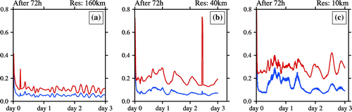
Figure 1 shows the temporal evolution of the relative numerical error of u_h at the middle layer of the atmosphere in different model resolutions, and Figure 2 is corresponding to that of w_h. The subscript ‘h’ means that the results are produced by the hydrostatic runs. The error measures used in this paper are defined as and , where means the true solution given by the NHDS and denotes the area-weighted average of q. From the given results, we can observe the following facts: First, the relative numerical error of u_h is not evident with an order of magnitude of 10⁻⁴–10⁻³ (see Figure 1), while for w_h the error is much more significant with an order of magnitude of 10⁻¹ (see Figure 2). Second, the error of w_h becomes more significant as model resolution increases. A similar trend can also be observed for u_h, although it is not as evident as that of w_h (see Figures 1 and 2). The above facts imply that the hydrostatic approximation (i.e. S ≡ 0) primarily influences w, which is one of the variables that is closely related with the vertical motion of the atmosphere. Other variables, such as u, however, show insensitive responses to the influence of S. Moreover, higher model resolution amplifies the impacts of non-hydrostatic perturbations on both u and w.

Figure 1. Temporal evolution of the relative numerical error of u_h at the mid-layer of the atmosphere under different model resolutions: (a) 160 km; (b) 40 km; (c) 10 km.

Note: Blue: E₁; Red: E₂.

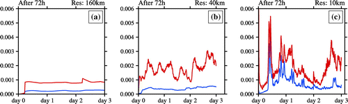
Figure 2. Temporal evolution of the relative numerical error of w_h at the mid-layer of the atmosphere under different model resolutions: (a) 160 km; (b) 40 km; (c) 10 km.

Note: Blue: E₁; Red: E₂.

The numerical results, together with the qualitative analysis in the previous paragraphs, motivates us to handle the impacts of non-hydrostatic perturbations by focusing our efforts on the vertical aspect of the atmosphere. Furthermore, as is shown in the above analysis, the impacts of non-hydrostatic perturbations can be quantified by a single term (i.e. S) in the vertical momentum equation. Therefore, they might be captured in a unified manner with less consideration of the particular formulation of a dynamics solver, if S could be approximated via some well-designed approaches.

2.2. Method

Following the motivation in the above subsection, a new approach is proposed in this paper to incorporate non-hydrostatic features into the current HDS. In order to illustrate the approach, Equation (1(1) ) is transformed as follows:(3)

The central task of the approach lies in estimating Sⁿ⁺¹ for the current integration step. Note that S⁰, S¹, …, Sⁿ can be exactly calculated via its definition, and hence it is natural to utilize these values to construct an estimator for Sⁿ⁺¹. Using the notations and terminologies from time series theory, the estimation problem can be formalized as follows: First, the sequence Sⁱ (i = 0, 1, …, n) is defined as an information set (Box, Jenkins, and Reinsel 2008). Then, the problem of estimating Sⁿ⁺¹ now becomes(4)

where represents an estimator of Sⁿ⁺¹ based on all available information about S up to time-step n. This equation can be interpreted in several ways according to which perspective is taken. For instance, if a stochastic view is taken at the sequence Sⁱ (i = 0, 1, …, n), then the E in Equation (4(4) ) can be recognized as an expectation operator. On the other hand, if the sequence Sⁱ (i = 0, 1, …, n) is treated as deterministic, then the E in Equation (4(4) ) becomes an ordinary extrapolation operator. Therefore, a wide variety of choices are available as to the sub-model used to estimate Sⁿ⁺¹.

No matter which sub-model is adopted, it must comply with some common restrictions. For instance, the following requirement must be satisfied for all candidate sub-models:(5)

Here, represents a null information set that contains only values of 0. The above restriction actually means that S will go to zero identically at all time steps if a null information set is given. Hence, the adjustment for the impacts of non-hydrostatic perturbations will be turned off given a null initial information set. On the contrary, if the adjustment is to be turned on, then the given initial information set must contain a valid signal about non-hydrostatic perturbations, or in other words has to be compatible with the full atmospheric dynamics including non-hydrostatic features. Thus, the adjustment can be automatically switched on and off in the modified dynamics solver (MDS) via feeding in different initial information sets.

However, the initial information sets containing the signal of non-hydrostatic perturbations do not exist before starting model integrations. So, they must be generated by some specialized utilities in cases where the adjustment is required to take effect. Since the WRF model has already implemented a well-functioned NHDS, it is natural to utilize it to accomplish this task. As a result, the standard NHDS built in the model may serve as an initialization utility for the MDS.

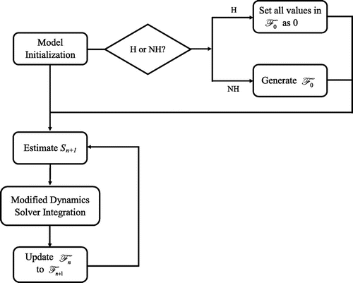
So far, the general framework of the approach has been established, as illustrated in Figure 3. Using this framework, we are able to experiment with and evaluate various types of sub-models for the impacts of non-hydrostatic perturbations. Via judiciously choosing the sub-model used in Equation (4(4) ), the impacts of non-hydrostatic perturbations can be captured without having to solve a complicated set of PDEs using time-consuming numerical integration procedures. Furthermore, the framework provides a flexible treatment of non-hydrostatic perturbations that can be conveniently applied to existing hydrostatic atmospheric models, especially those for climate simulations.

Figure 3. Framework of the approach.

Note: H: hydrostatic; NH: non-hydrostatic.

3. Results

Although the general framework of the approach has been laid down, the particular form of the estimator for Sⁿ⁺¹ in Equation (4(4) ) is still not given. In this paper, Equation (4(4) ) is replaced with the following equation:(6)

Here, is the intercept term, and , are respectively the coefficients for the terms of and . In Equation (6(6) ), a pointwise linear sub-model is employed to estimate Sⁿ⁺¹. The parameters in this model can be dynamically estimated using the updated information set at each time step. For simplicity, they are prescribed as for all i, j, k, n. Thus, the estimator for can be split into two parts: and , the latter of which is a simple local estimate of the trend of S.

To preliminarily verify the approach, the previous test case was repeated with the model resolution set to 10 km. The same model configurations as the former runs were used except that the MDS was employed. The results of this run are again compared with the true solution given by the non-hydrostatic run with the same model resolution. Figure 4 shows the temporal evolution of the relative numerical error of u_m at the middle layer of the atmosphere, and Figure 5 illustrates that of w_m. The subscript ‘m’ means that the results are given by the MDS.

Figure 4. Temporal evolution of the relative numerical error of u_m at the mid-layer of the atmosphere.

Note: Blue: E₁; Red: E₂.

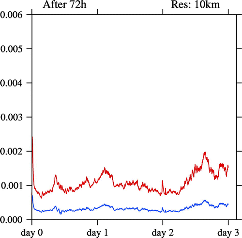
Figure 5. Temporal evolution of the relative numerical error of w_m at the mid-layer of the atmosphere.

Note: Blue: E₁; Red: E₂.

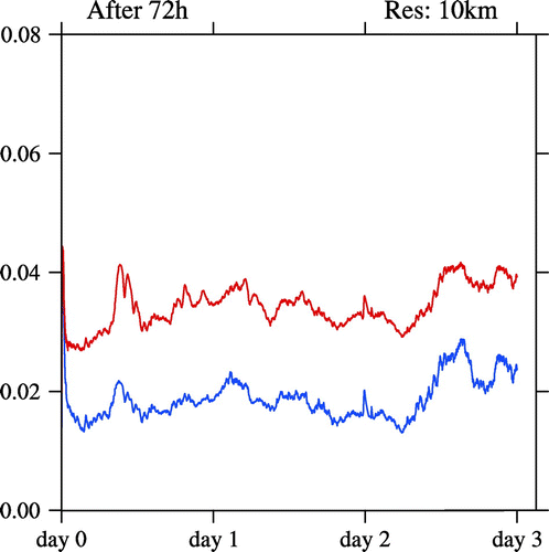
It is easy to see that the numerical error of the MDS is reduced successfully by the approach compared with that of its hydrostatic predecessor. For u_m, the numerical error is somewhat suppressed, although the improvement is not very evident (see Figures 1(c) and 4). For w_m, the numerical error is significantly reduced by about 80%–90% from the order of magnitude of 10⁻¹–10⁻² (see Figures 2(c) and 5). Therefore, the impacts of non-hydrostatic perturbations are basically captured in the MDS. However, as its hydrostatic predecessor, the numerical error of w_m (~10⁻²) is still much larger in magnitude than that of u_m (~10⁻⁴) (see Figures 4 and 5). Furthermore, in contrast with Figures 1(c) and 2(c), the curves in Figures 4 and 5 show more stabilized patterns with fewer large spikes that are yielded by relatively large deviations from the true solution. Overall, the MDS replicates to a large extent the simulation results of the standard NHDS built in the WRF model. Furthermore, the main source of the numerical error of the MDS, albeit greatly suppressed, still comes from w_m, urging us to refine the sub-model for the impacts of non-hydrostatic perturbations employed in this study.

The above results are not hard to explain. As pointed out in the previous section, the term S, representing the impacts of non-hydrostatic perturbations, appears in the vertical momentum equation, and thus it has an immediate connection with the vertical motion of the atmosphere. So, the estimated S is used to directly correct the numerical results for variables that have a significant dependence on the vertical motion of the atmosphere (e.g. w). The correction effects are then transferred to other variables (e.g. u) via the interactions between variables in the MDS. However, these variables are generally dominated by the large-scale dynamics of the atmosphere. Hence, they are not as sensitive to the impacts of non-hydrostatic perturbations as the aforementioned variables.

4. Discussion and conclusion

Non-hydrostatic perturbations have increasingly prominent influences on the dynamics of the atmosphere as the resolution of atmospheric models becomes higher. Current approaches to handling their impacts in NHDSs for high-resolution atmospheric models are very time-consuming and too complicated to be applied to existing hydrostatic atmospheric models, especially those for climate simulations. To investigate the impacts of non-hydrostatic perturbations, this study analyzed the differences between HDSs and NHDSs using the WRF model as an example. The analysis revealed that non-hydrostatic perturbations mainly influenced variables that had a close relation with the vertical aspect of the atmosphere, and that their impacts could be represented by a single term in the full vertical momentum equation without the hydrostatic approximation.

The analysis motivated a flexible approach to adjusting the HDS for the impacts of non-hydrostatic perturbations, so as to enable them to function equivalently as non-hydrostatic models. The approach employed a separate sub-model to estimate the impacts of non-hydrostatic perturbations on the current integration step based on the information obtained from previous time steps. In contrast with traditional treatments of non-hydrostatic perturbations, the approach circumvented time-consuming computational procedures to integrate complicated sets of PDEs. Moreover, the framework underlying the approach was flexible enough to be easily adopted in other hydrostatic atmospheric models besides the one used in this paper. Furthermore, using the approach, the adjustment for the impacts of non-hydrostatic perturbations was provided as an optional feature in the MDS, which could be automatically enabled or disabled by feeding in different initial information sets. The approach was preliminarily tested on the WRF model by running the 3d baroclinic-wave test case. Results showed that the MDS behaved quite closely to the standard NHDS, rather than its hydrostatic predecessor, indicating that the impacts of non-hydrostatic perturbations were basically captured by the approach.

On the other hand, it should be noted that many aspects of the approach need to be refined. For instance, the sub-model used in Equation (4(4) ) ought to be optimized to obtain a better estimation of the impacts of non-hydrostatic perturbations. In addition, other techniques than that adopted in this study should also be pursued to generate initial information sets, including non-hydrostatic features of the atmosphere. Therefore, further research will be done to resolve these issues in the future.

Disclosure statement

No potential conflict of interest was reported by the authors.

Funding

This work was supported by the National Key Research and Development Program [grant number 2016YFB0200805] and the National Natural Science Foundation of China [grant number 41622503].

References

- Box, G. E., G. M. Jenkins, and G. C. Reinsel. 2008. Time Series Analysis: Forecasting and Control. 4th ed. Hoboken, NJ: Wiley.10.1002/9781118619193
- Cheng, R. 2010. “Design of the AREM-Based Non-Hydrostatic Model and Its Application in Typhoon Simulation.” [In Chinese.] PhD diss., Graduate University of Chinese Academy of Sciences.
- Clark, T. L. 1977. “A Small Scale Numerical Model Using a Terrain following Coordinate System.” Journal of Computational Physics 24 (2): 186–215.10.1016/0021-9991(77)90057-2
- Donner, L. J., B. L. Wyman, R. S. Hemler, L. W. Horowitz, Y. Ming, M. Zhao, J. Golaz, et al. 2010. “The Dynamical Core, Physical Parameterizations, and Basic Simulation Characteristics of the Atmospheric Component AM3 of the GFDL Global Coupled Model CM3.” Journal of Climate 24 (13): 3484–3519. doi:10.1175/2011JCLI3955.1.
- Erbes, G. 1993. “A Semi-lagrangian Method of Characteristics for the Shallow-water Equations.” Monthly Weather Review 121 (12): 3443–3452. doi:10.1175/1520-0493(1993)121<3443:ASLMOC>2.0.CO;2.
- Hall, D. M. 2013. “A Nonhydrostatic Atmospheric Dynamical-Core for Climate Modeling.” Paper presented at the AGU Fall Meeting 2013, San Francisco, December 9–13.
- Jablonowski, C., and D. L. Williamson. 2006. “A Baroclinic Instability Test Case for Atmospheric Model Dynamical Cores.” Quarterly Journal of the Royal Meteorological Society 132 (621C): 2943–2975. doi:10.1256/qj.06.12.
- Klemp, J. B., and R. B. Wilhelmson. 1978. “The Simulation of Three-dimensional Convective Storm Dynamics.” Journal of the Atmospheric Sciences 35 (6): 1070–1096. doi:10.1175/1520-0469(1978)035%3C1070:TSOTDC%3E2.0.CO;2.
- Lauritzen, P. H., C. Jablonowski, M. A. Taylor, and R. Nair. 2011. Numerical Techniques for Global Atmospheric Models. New York: Springer.10.1007/978-3-642-11640-7
- Peng, X. D., and X. L. Li. 2010. “Advances in the Numerical Method and Technology of Multi-scale Atmospheric Prediction.” [in Chinese.] Journal of Applied Meteorological Science 21 (2): 129–138. doi:10.11898/1001-7313.20100201.
- Satoh, M., T. Matsuno, H. Tomita, H. Miura, T. Nasuno, and S. Iga. 2008. “Nonhydrostatic Icosahedral Atmospheric Model (NICAM) for Global Cloud Resolving Simulations.” Journal of Computational Physics 227 (7): 3486–3514. doi:10.1016/j.jcp.2007.02.006.
- Skamarock, W. C., Klemp, J. B., Dudhia, J., Gill, D. O., Barker, D. M., Duda, M. G., Huang, X. Y., Wang, W., and Powers, J. G. 2008. A Description of the Advanced Research WRF Version 3. NCAR Technical Note NCAR/TN-475+STR.
- Smolarkiewicz, K., C. Kühnlein, and N. Wedi. 2014. “A Consistent Framework for Discrete Integrations of Soundproof and Compressible PDEs of Atmospheric Dynamics.” Journal of Computational Physics 263 (8): 185–205. doi:10.1016/j.jcp.2014.01.031.
- Tapp, M. C., and P. W. White. 1976. “A Non-hydrostatic Mesoscale Model.” Quarterly Journal of the Royal Meteorological Society 102 (432): 277–296. doi:10.1002/qj.49710243202.