Impact of Kuroshio Extension dipole mode variability on the North Pacific storm track

Abstract

An index of a large-scale Kuroshio Extension (KE) sea surface height dipole (KED) mode is constructed using satellite altimeter sea level anomaly observations from January 1993 to December 2015 based on previous work of the second author. It is found that the KED mode that undergoes a decadal variation from a negative phase (a positive-over-negative dipole, KED⁻) to a positive phase (a negative-over-positive dipole, KED⁺) can affect the variability of the oceanic SST front and the North Pacific storm track. The results show that the oceanic SST fronts in the north of the KE region and in the KE region — referred to as the NSST and KSST fronts, respectively — are closely correlated with the KED mode. In the NSST front region, the SST front is stronger for KED⁻ than for KED⁺, and the opposite is the case in the KSST region. It is further revealed that the decadal phase transition of the KED mode can change the location and strength of the North Pacific storm track, with the North Pacific storm track being slightly weaker and moving more northwards as a whole during the KED⁻ mode than during the KED⁺ mode. The westerly wind associated with the storm track on the downstream side of the KE region intensifies and shifts northwards under KED⁻ compared to KED⁺. Furthermore, the transition of the KED mode gives rise to changes in the North Pacific storm track by changing the NSST and KSST fronts and meridional heat flux.

摘要

利用1993年1月至2015年12月的海表面高度异常资料引入黑潮延伸体偶极子模态指数（KED模指数），发现KED模存在正位相（南正北负偶极子模态）和负位相（南负北正偶极子模态）之间的年代际变化，并对海洋锋和北太平洋风暴轴产生影响。研究结果显示，黑潮延伸体北侧海洋锋和延伸体海洋锋都与KED模存在很好的相关关系。在黑潮延伸体北侧海洋锋区域，KED负模态下海洋锋的强度增强，延伸体区域海洋锋则相反。另外在KED负模态下，风暴轴会减弱北移，与风暴轴有关的西风也在风暴轴下游区域北移。进一步分析得到KED模态的转换可以改变海洋锋的强度从而改变上空经向热量通量，进而影响风暴轴。

Keywords:

• Kuroshio Extension
• oceanic front
• North Pacific storm track

关键词:

• 黑潮延伸体
• 海洋锋
• 北太平洋风暴轴

1. Introduction

The Kuroshio Extension (KE) is the eastward jet extension region where the western boundary current loses the support from the Japan coast (Mizuno and White 1983). Qiu and Chen (2005) noted by using sea surface height (SSH) data that the KE system shows a clear decadal variability. It is recognized that the first and second modes of the empirical orthogonal function (EOF) — EOF1 and EOF2, respectively — reflect the annual and decadal variations of the KE system; specifically, EOF2 describes the variations of the southern recirculation gyre with a periodicity of 8–10 years. It has also been suggested that the decadal variations of the southern recirculation gyre are associated with the Pacific Decadal Oscillation (Pan, Zhang, and Lin 2012; Li et al. 2015). Considering the strong nonlinearity of the KE system, the linear EOF method cannot describe the nonlinear variability of the KE system effectively. Hence, a more effective index is needed to represent the KE variability. Recently, Luo, Feng, and Wu (2016) constructed a KE SSH dipole (KED) index to reflect the KE decadal variation from a weaker to a stronger meandering.

It has been revealed that the sensible heating across the SST front enhances baroclinicity, and this change can reach the troposphere and, ultimately, affects the storm track (Nakamura et al. 2004). Moreover, the SST front in the midlatitude zone can influence the location and strength of the Pacific storm track, especially its latitude (Chen, Plumb, and Lu 2010; Ma and Xu 2012; Ogawa et al. 2012). Therefore, change in the SST front in the KE region may be a key factor for change in the Pacific storm track. There is a significant correlation between a strong SST front in the northern KE region and the strength of the KE (Chen 2008). As demonstrated in Luo, Feng, and Wu (2016), the phase of the large-scale KED mode can better represent the variability of the KE system. Thus, it is meaningful to examine how the variation of the KED mode affects the SST front and subsequently the Pacific storm track, which is the purpose of the present paper.

2. Data and methods

To characterize the variability of the KE, we use daily sea level anomaly (SLA) data from the AVISO data center (https://www.aviso.altimetry.fr/en/home.html). To characterize the oceanic front, we use daily sea surface temperature (SST) data from Met Office Hadley Centre (https://www.metoffice.gov.uk/hadobs/hadisst/index.html) observations at a resolution of 1° × 1° from January 1993 to December 2015. On this basis, we use the SST data to calculate the SST gradient,

to represent the strength of the oceanic front, where T is the SST and y is the north-south coordinate.

The daily reanalysis data of height, wind, and temperature fields are from the National Centers for Environmental Prediction/National Center for Atmospheric Research (https://www.esrl.noaa.gov/psd/data/gridded/data.ncep. reanalysis.html), with 2.5° × 2.5° grid points, from January 1993 to December 2015. The synoptic eddy kinetic energy (EKE) at the 300-hPa level, which is within a timescale of 2.5–7 days and can be calculated using a second-order Butterworth filter, is used to represent the North Pacific storm track. In order to understand the relationships among the Pacific storm track, oceanic front, and KED mode, correlation and composite analysis are used.

3. Results

3.1. Variation of the KE system

We begin by using EOF analysis to extract the characteristic patterns of the SLA in the midlatitude North Pacific region (25°–45°N, 130°–160°E) from January 1993 to December 2015. Before calculation, however, we de-trend the data and use the daily SLA minus the climate-mean SLA on that day to remove the seasonal change in the SLA data. Figure 1(a) and (b) show the EOF1 and EOF2 components of the SLA, and Figure 1(c) and (d) the time series of their corresponding PC1 and PC2. The calculation shows that the variance percentages of EOF1 and EOF2 are 9.5% and 7.2%, respectively. It is further found that the EOF1 spatial pattern exhibits a wave train structure with positive, negative, and positive height anomalies from the southwest–northeast to northwest–southeast direction in the KE region (Figure 1(a)). EOF2 exhibits a strong positive-over-negative dipole anomaly structure in the meridional direction at 144°E. The PC1 time series shows a clear decadal variation with a period of 10 years, but PC2 exhibits a clear interannual variability with a 2–4-year periodicity, and a less-distinct decadal variability with a secondary periodicity of 8–10 years, as revealed from a power spectral calculation (data not shown). Although EOF2 shows a clear dipole structure, its PC time series does not possess a strong decadal variability. However, the EOF1 pattern does not have a typical dipole structure, while its PC1 time series has a clear decadal variability. For this reason, as in (Luo, Feng, and Wu (2016), we calculate the area-averaged low-frequency SSH anomalies over (32°–35°N, 141°–153°E) and (35°–38°N, 141°–153°E) and define their difference as an index to reflect the variability of the dipole anomaly in phase and strength existing in the KE region — hereafter referred to as the KED mode index. Such a definition avoids using linear EOF decomposition to extract the signal of the KE decadal variability. Based on 0.4 standard deviations of the normalized KED index time series, as shown in Figure 1(g), the value for ≥0.4 (≤−0.4) of the normalized KED index is defined as a KED⁺ (KED⁻) index, which includes 23 (24) winter months during 1993–2015. We perform a composite analysis of the SLA for the positive and negative phases of the KED and show its result in Figure 1(e) and (f). It is found that KED⁺ has a negative-over-positive dipole structure (Figure 1(e)), and the opposite pattern is found for KED⁻ (Figure 1(f)). Comparing Figure 1(a) and (b) reveals that the KED mode can better reflect the spatial structure of the dipole mode and its decadal variability (Figure 1(g)).

Figure 1. (a, b) Spatial patterns of the (a) EOF1 and (b) EOF2 of the SLA anomalies (units: m). (c, d) The corresponding normalized time coefficients ((c) PC1 and (d) PC2) for the EOF1 and EOF2 of the SLA anomalies. (e, f) Composite distributions of the SSH anomalies of the (e) KED⁺ mode and (f) KED⁻ mode (units: m). (g) Time series of normalized monthly mean KED index from January 1993 to December 2015. The red thick line denotes the 11-month smoothing curve.

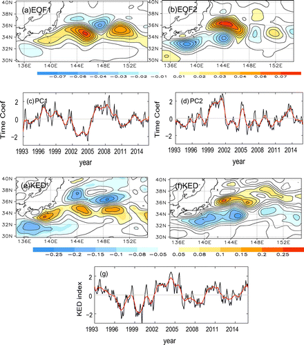
It is important to note that, if the KED index is positive, it corresponds to less meandering, and vice versa (Luo, Feng, and Wu 2016). As such, one can examine the impact of KE meandering on the Pacific storm track through investigating the effect of the KED mode.

3.2. Relationship between the oceanic SST front and the KED mode

It is well-known that an obvious oceanic SST front occurs in the north of the KE region. Climatologically, the oceanic SST front is located at about 40°N, north of the KE region. Some studies have indicated that the Pacific storm track is influenced by the variability of the oceanic SST front in the KE region (Nakamura et al. 2004; Chen, Plumb, and Lu 2010; Ma and Xu 2012; Ogawa et al. 2012; Feng, Luo, and Zhong 2015). Thus, the KED can affect the Pacific storm track through a change in the oceanic SST front, which motivates us to establish a link between the oceanic SST front and the phase of the KED mode. First, we show the composite distributions of the oceanic SST of the KED⁺ mode, the KED⁻ mode, and the difference (KED⁻ minus KED⁺) in Figure 2(a)–(c). It is apparent that the high SST is shifted more northwards under the KED⁻ mode than under the KED⁺ mode (Figure 2(a) and (b)), and this is clear from the difference between them (KED⁻ minus KED⁺; Figure 2(c)). To further examine the influence of the KED mode on the oceanic front, it is useful to carry out a composite analysis of the SST gradient,

Figure 2. (a–c) Composite distributions of oceanic SST for the months of the (a) KED⁺ mode, (b) KED⁻ mode, and (c) the KED⁻ minus KED⁺ difference (units: °C). (d–f) Composite distributions of oceanic SST gradient for the months of the (d) KED⁺ mode, (e) KED⁻ mode, and (f) the KED⁻ minus KED⁺ difference (units: °C/100 km). Areas within red contours are statistically significant at the greater than 90% confidence level based on a two-sided Student’s t-test.

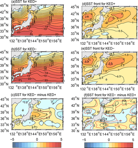
The distribution of the composite winter-mean oceanic SST front is shown in Figure 2(d) and (e) for the two phases of the KED mode. It is apparent that a major change in the oceanic front from KED⁺ to KED⁻ is its intensity, wherein its central intensity can reach 2.5 °C/100 km for KED⁻ (Figure 2(d) and (e)). Their difference field (KED⁻ minus KED⁺) shows a north–south dipole, with a positive center at 40°N and a negative center at 36°N (Figure 2(f)). This reflects that the oceanic SST front is stronger and located more north when the KED mode is in a negative phase.

To further understand whether the variation in the oceanic SST front is modulated by the KED mode, we define the oceanic temperature gradient,

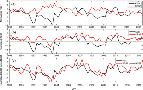
averaged over the region (38°–42°N, 141°–153°E) as the NSST front strength, and over the region (34°–38°N, 141°–153°E) as the KSST front strength. The time series of the normalized winter monthly mean KED index, NSST and KSST front strengths, and the NSST minus KSST difference, are shown in Figure 3. We can see that the KED index exhibits a clear decadal variation and has correlation coefficients of −0.53, 0.70, and 0.67 with the NSST front strength (Figure 3(a)), KSST front strength (Figure 3(b)), and their difference (Figure 3(c)), respectively. Obviously, the KED mode and the NSST (KSST) front strength have a significant negative (positive) correlation. In fact, the decadal variation of the SST front can be better explained by the phase of the KED mode. This is because warm water intrudes northwards when the KED is in a negative phase, and vice versa for a positive phase. This suggests that the presence of the KED⁻ mode can strengthen the SST front in the north of the KE region and make it shift northwards; whereas, the KED⁺ mode only favors the SST front in the KE region. Thus, we conclude that the phase of the KED mode can better reflect the variability of the SST front in strength and position over the KE region.

Figure 3. Time series of normalized winter monthly mean (a) NSST front strength, (b) KSST front strength, and (c) the KSST minus NSST differences, during the period 1993–2015. Black thick lines denote the KED index.

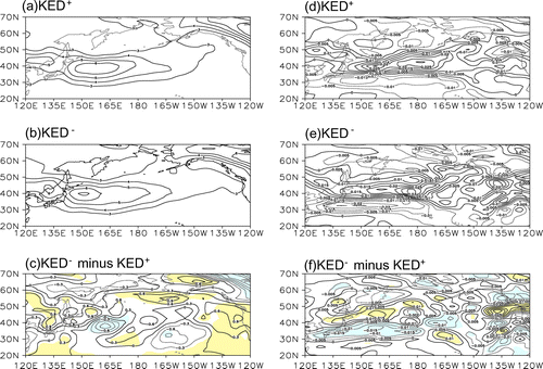
3.3. Impacts of the KED on the North Pacific storm track

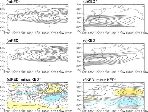
As noted above, because the KED can reflect the SST front variability in the KE region, it is valuable to examine how the phase of the KED affects the Pacific storm track through the SST front change. We show a composite analysis of the monthly-mean 300-hPa EKE in winter in Figure 4(a) and (b) for KED⁻ and KED⁺ months. It is apparent that the maximum center of the storm track shifts northeastwards to the Northeast Pacific under KED⁻ (Figure 4(b)), whereas the strongest Pacific storm track is mainly confined to the central North Pacific under KED⁺ (Figure 4(a)). Their difference clearly indicates this point (Figure 4(c)). Thus, it can be concluded that a change in the phase of the KED mode can affect the Pacific storm track. This point is easily explained through the zonal wind change, because the storm track change is significantly influenced by the strength of the westerly jet. When the Pacific westerly jet is stronger, the Pacific storm track is also stronger. As such, we can understand how the KED mode affects the Pacific storm track if the impact of the KED mode on the westerly jet can be known. Accordingly, we show the composite monthly mean 300-hPa westerly wind fields in winter for the KED⁺ and KED⁻ modes in Figure 4(d) and (e), and their difference in Figure 4(f). It is apparent that, because the westerly jet is stronger under KED⁻ (Figure 4(e)) than under KED⁺ (Figure 4(d)), the Pacific storm track is stronger and shifts more northeastwards under KED⁻ than under KED⁺. Thus, the northeastward-intensified Pacific storm track is possibly a result of the enhanced North Pacific westerly jet related to the intensified northward-shifted SST front in the KED⁻ mode. To the best of the authors’ knowledge, this is a new finding.

Figure 4. (a, b) Composite distributions of the 300-hPa EKE of the (a) KED⁺ mode, (b) KED⁻ mode, and (c) the KED⁻ minus KED⁺ differences (units: m² s⁻²). (d–f) Composite distributions of the 300-hPa westerly jet of the (d) KED⁺ mode, (e) KED⁻ mode, and (f) the KED⁻ minus KED⁺ difference (units: m s⁻¹). Shading denotes the 95% confidence level for a two-sided Student’s t-test.

To understand why the phase of the KED mode can affect the North Pacific westerly jet, and then the Pacific storm track, we need to calculate the meridional eddy heat flux anomaly. Considering (Liu and Liu 2011)

and

where is the mean westerly wind; and are the eddy meridional wind and zonal wind, respectively; is a positive constant; and is the mean air temperature for a given level, it is easy to estimate the contribution of the meridional eddy heat flux and momentum flux to the westerly wind and its baroclinicity for the two phases of the KED mode by calculating and .

The composite 850-hPa meridional eddy heat flux is shown in Figure 5(a) and (b) for the KED⁻ and KED⁺ months. We can see that the meridional eddy heat flux is stronger on the north side of the KE system for the KED⁻ mode than for the KED⁺ mode, and this is further apparent from their difference field (Figure 5(c)). In terms of the thermal wind relationship, it is easy to obtain . As such, it can be concluded that, when the meridional eddy heat flux is stronger, the vertical wind shear is stronger, and produces a stronger storm track in the northeastern Pacific. It is also noted that matches the spatial distributions of the EKE and westerly wind. Thus, we can conclude that the strong storm track is due to the stronger meridional eddy heat flux, through an intensified vertical wind shear, when the intensified SST front shifts northwards during the KED⁻ period.

Figure 5. (a, b) Composite distributions of the 850-hPa meridional eddy heat flux of the (a) KED⁺ mode, (b) KED⁻ mode, and (c) the KED⁻ minus KED⁺ differences (units: K (m s⁻¹)⁻¹). (d–f) Composite distributions of gradient of the 300-hPa meridional momentum flux of the (d) KED⁺ mode, (e) KED⁻ mode, and (f) the KED⁻ minus KED⁺ differences (units: m s⁻²). Shading denotes the 95% confidence level for a two-sided Student’s t-test.

The monthly mean is shown in Figure 5(d) and e for the KED⁻ and KED⁺ months. We can see that is mostly positive and stronger for the KED⁻ mode than for the KED⁺ mode — a feature clearly reflected in their difference in Figure 5(f). Thus, the NSST front during the KED⁻ period can strengthen the North Pacific storm track through enhancing the westerly wind and its vertical shear on the northeast side of the KE region.

4. Conclusions

In this study, we define a KED index that reflects the large meandering of the KE jet to examine the impact of KE meandering on the Pacific storm track. It is demonstrated that the phase of the KED mode can better reflect the decadal variability of the oceanic SST front in the KE system. On this basis, the impact of the KED mode on the Pacific storm track is examined. The main new conclusions are as follows:

(1)

The oceanic SST front, in strength and position, is modulated by the phase of the KED mode. For the KED− mode, the SST front is intensified and displaced northwards due to the northward intrusion of warm water across the KE jet core. But, for the KED+ mode the intensified SST front is mainly located in the KE region.

(2)

For the KED− mode, the westerly jet and its vertical shear in the North Pacific, downstream of the KE, are intensified such that a strong Pacific storm track is produced because the meridional eddy heat flux, with being positive, is strong on the north side due to the intensified northward-shifted SST front. The opposite situation is found for the KED+ mode. Thus, the decadal transition of the KED phase can affect the location and strength of the North Pacific storm track through changing the oceanic SST front in strength and meridional position.

However, it should be noted that, although the Pacific storm track is significantly influenced by the phase of the KED mode, it is unclear how changes in the large-scale atmospheric circulations in the North Pacific are linked to the decadal variability of the KED mode. This deserves further investigation.

Disclosure statement

No potential conflict of interest was reported by the authors.

Funding

This work was supported by the National Basic Research Program of China [grant number 2013CB956203] and the National Natural Science Foundation of China [grant number 41490642].

References

- Chen, S. 2008. “The Kuroshio Extension Front from Satellite Sea Surface Temperature Measurements.” Journal of Oceanography 64: 891–897. doi:10.1007/s10872-008-0073-6.
- Chen, G., R. A. Plumb, and J. Lu. 2010. “Sensitivities of Zonal Mean Atmospheric Circulation to SST Warming in an Aqua-Planet Model.” Geophysical Research Letters 37: 245–269. doi:10.1029/2010GL043473.
- Feng, S., D. Luo, and L. Zhong. 2015. “The Relationship between Mesoscale Eddies in the Kuroshio Extension Region and Storm Tracks in the North Pacific.” Chinese Journal of Atmospheric Sciences 39: 861–874.
- Li, J., L. Du, F. Han, Q. Zhang, and F. Ye. 2015. “Inter-Annual Sea Level Variation and Its Relationship with Kuroshio Current in the Kuroshio Extension.” Marine Science Bulletin 34: 158–167.
- Liu, S., and S. Liu. 2011. Atmospheric Dynamics. Beijing: Peking University Press.
- Luo, D., S. Feng, and L. Wu. 2016. “The Eddy-Dipole Mode Interaction and the Decadal Variability of the Kuroshio Extension System.” Ocean Dynamics 66: 1317–1332. doi:10.1007/s10236-016-0991-6.
- Ma, J., and H. Xu. 2012. “The Relationship between Meridional Displacement of the Oceanic Front in Kuroshio Extension during Spring and Atmospheric Circulation in East Asia.” Journal of the Meteorological Sciences 32: 375–384.
- Mizuno, K., and W. B. White. 1983. “Annual and Interannual Variability in the Kuroshio Current System.” Journal of Physical Oceanography 13: 1847–1867.10.1175/1520-0485(1983)013<1847:AAIVIT>2.0.CO;2
- Nakamura, H., T. Sampe, Y. Tanimoto, and A. Shimpo 2004. “Observed Associations among Storm Tracks, Jet Streams and Midlatitude Oceanic Fronts.” In Earth’s Climate: The Ocean–Atmosphere Interaction, edited by C. Wang, S.-P. Xie, and J. A. Carton, 329‒345. Geophys Monogr 147. Washington, DC: AGU.
- Ogawa, F., H. Nakamura, K. Nishii, T. Miyasaka, and A. Kuwano-Yoshida. 2012. “Dependence of the Climatological Axial Latitudes of the Tropospheric Westerlies and Storm Tracks on the Latitude of an Extratropical Oceanic Front.” Geophysical Research Letters 39: 578–594. doi:10.1029/2011GL049922.
- Pan, F., Y. Zhang, and M. Lin. 2012. “Spatial and Temporal Variability of the Sea Level Anomalies and Mesoscale Eddies in the Region of the Kuroshio Extension.” Marine Forecasts 29: 29–38.
- Qiu, B., and S. Chen. 2005. “Variability of the Kuroshio Extension Jet, Recirculation Gyre, and Mesoscale Eddies on Decadal Time Scales.” Journal of Physical Oceanography 35: 2090–2103. doi:10.1175/JPO2807.1.