Ensemble transform sensitivity for adaptive observations: a general formulation and its practicable implementation

ABSTRACT

The Ensemble Transformation (ET) method and its variation ET-based Sensitivity (ETS) method have been used in adaptive observation studies. However, the solution of the ensemble transformation matrix in the ET and ETS methods is not unique. A general mathematical formulation for the ensemble transformation matrix is derived and then a generalized equation for the ETS method is derived. It is proved that the previous ETS formulation is a special implementation of the newly derived general formulation. Another practicable implementation of the general ETS formulation that avoids calculating the inverse of some matrices is proposed. This ETS implementation showed physically reasonable statistical sensitivity regions for improving 1–3 day weather forecasts over eastern regions of U.S.A and Beijing region, China.

KEYWORDS:

• Adaptive observations
• ensemble transform
• sensitivity analysis

1. Introduction

Adaptive observations have been employed in field campaigns to increase forecast accuracy of high-impact weather events. One of key factors in adaptive observations is to provide guidance of data sensitive region for collecting additional observations in a few days ahead of the high-impact weather events. In addition to several adjoint-based methods, such as the singular vector method (SVs; Palmer et al. 1998; Buizza and Montani 1999) and the conditional nonlinear optimal perturbation method (Mu, Zhou, and Wang 2009; Wang, Mu, and Huang 2011; Yu et al. 2017), ensemble-based methods, such as the ensemble transformation method (ET; Bishop and Toth 1999, hereafter BT1999) and the ensemble transform Kalman filter method (ETKF; Bishop, Etherton, and Majumdar 2001) are also widely applied in field campaigns (Chang, Zheng, and Raeder 2013; Xie et al. 2013). Compared to the adjoint-based methods, the ensemble-based methods do not require adjoint models and are also less computationally demanding (Ancell and Hakim 2007; Ito and Wu 2013).

Among the ensemble-based methods, the ET method proposed by Bishop and Toth (1999) provides a practicable approach for adaptive observations. In a recent research, an ET-based sensitivity (ETS) method was proposed by Zhang et al. (2016, hereafter Z2016) to specify sensitive area for adaptive observations. The ETS method calculates the gradient of forecast error variance reduction in terms of analysis error variance reduction. The ETS method produces similar results to ET and reduces computational cost because only a single transformation matrix calculation is required.

In this letter, it is showed that the solution of the ensemble transformation matrix in is not unique, and thus the previous study (BT1999 and Z2016) may potentially provide a suboptimal solution. A general mathematical formulation of the ensemble transformation matrix and a general formulation of the ETS method are derived and described. The general ETS formulation provides a basis for further investigating other kind of practical solutions and uncertainties caused by choosing different transformation matrices. This paper is organized as follows. In section 2, a precise review on the ET method and a general formulation of the transform matrix are presented. In section 3, a general ETS formulation is described. And it is shown that the ETS formulation in Z2016 is a special implementation of the general solution. Another more practicable implementation of the general ETS formulation is introduced, which has merits of avoiding inverse process of a matrix and its applications in some cases are also presented. A summary is provided in the final section.

2. ET method and a new formulation for ensemble transform matrix

2.1. ET method

First, a precise description on the ET method (BT1999) is presented before introducing the ETS method. Assuming an ensemble of forecasts perturbations (ensemble forecasts minus ensemble mean) over a period is available. Let X^a denotes ensemble perturbations at a future sensitivity analysis time before assimilating a set of the adaptive observations, ensemble perturbations at a future verification time, and the ensemble perturbations after assimilating the adaptive observations. The idea of ensemble transformation is to present by introducing a transformation matrix C, such that

(1)

Here it is assumed that is a linear transformation from X^a. presents the analysis error covariance matrix after assimilating the adaptive observations for evaluation. C is a matrix. The matrixes X^a, , and are matrixes. Here is dimension of an ensemble state vector, and is number of member in the ensemble.

The transformation matrix C is also used to predict the ensemble-based forecast error covariance at verification time (P^v),

(2)

The C in the above two equations is required to approximate a known guessed analysis error covariance of A after assimilation the set of adaptive observations at the sensitivity analysis time,

(3)

A solution of C given in BT1999 is,

(4)

The above Equation (4) is used to predict the prediction error covariance defined by Equation (2). In order to estimate impact of the set of adaptive observations, two experiments are required, one control experiment that does not assimilate that set of observations and the other sensitivity experiment that assimilates that set of observation are required. Assuming is the guess error covariance for the control experiment at the sensitivity analysis time, and is the guess error covariance for the sensitivity experiment at the sensitivity analysis time, then the C matrices associated with the two experiments are,

(5a)

(5b)

In real applications, the inverse of the guess analysis error is difficult to be obtained. Following BT1999 and Majumdar et al. (2002), only the diagonal elements of analysis error covariance are considered to obtain the transformation matrix.

(6a)

(6b)

Here and are diagonal matrixes that only include diagonal elements of the analysis error covariance matrixes of and . Given the ensemble transformation matrix defined in Equations (5)–(6), the impact of the targeted data is evaluated by calculating the difference between the two prediction error covariances (P_diff),

(7)

It is seen that the ensemble transformation matrix needs to be calculated twice to evaluate the impact of the targeted observations. If thousands of potential observational locations or flight patterns for adaptive observations need to be evaluated, then thousands of calculations of the ensemble transformation matrix are required.

2.2 A general solution of ensemble transformation matrix C

BT1999 described a solution of C (Equation (4)) which had been used in the ETS formulation in Z2016. A careful investigation of Equation (3) showed that the solution for the ensemble transform matrix is not unique because the X^a, which is a non-square matrix, is not invertible. The previous applications (BT1999 and Z2016) may potentially provide a sub-optimal solution, instead of an optimal solution for targeted observations. A general solution for the ensemble transform matrix is described in this section.

Since ensemble perturbation matrix X^a can include different atmospheric variables, a symmetric matrix introduced to weight each element in the perturbation ensemble. W is a matrix. By multiplying and from the left and right of Equation (3),

(8)

Assuming the inverse of the symmetric square matrix exists, then

(9)

The above Equation (9) is a general formulation of the ET matrix. It is obvious that different implementations of the weighting matrix W will lead to the different ensemble transformation matrix.

It is proven that the solution of the ensemble transformation matrix (Equation (4)) defined in BT1999 is a special implementation of the general solution Equation (9). Provided that W is equal to the inverse of the guess analysis error covariance matrix A, , then

The above solution is exactly same to Equation (4) derived in BT1999. In another word, the ensemble transform matrix defined in BT1999 is a special implementation of the general solution Equation (9).

3. A general ETS formulation and its simplified implementation

3.1 A general ETS formulation

To objectively measure on the error reduction caused by assimilating a set of adaptive observations, usually a scalar response function is defined to measure the forecast errors reduction defined in Equation (7).

Mathematically, the response function is the sum of the diagonal elements of P_diff, where

(10)

Let

(11)

The vector a and b whose element , denotes the variance parts of analysis error matrixes of and . whose element is a parameter measuring an analysis error reduction ratio caused by assimilating the observations for evaluation. The maximum value of is 1.0. It means the analysis error variance becomes 0 after assimilating the observations for estimating impact.

The transformation matrix can be rewritten as

(12)

can be written as

(13)

where . The z_i is a row vector with columns. The matrix is introduced to represent an error metric (norm). For example, if a kinetic energy norm is used, then only the diagonal elements for u and v variables have values of 1. Other elements of are 0.

The idea of the ensemble transform sensitivity method (ETS) is to use the gradient of forecast error variance in terms of analysis error variance to determine data sensitive regions. The gradient of J to the analysis error variance reduction ratio is

(14)

Using general ensemble transformation matrix Equations (9) and (11), the general ETS formulation is written as,

(15)

Provided that analysis error matrix is not a function of W, it is obvious that the ETS signal is proportional to amplitude of analysis error variance because . In other words, ETS intends to identify region of larger analysis error variance as data sensitive area. This feature is physically meaningful because that targeted observations need to be placed in regions where the analysis errors have room to be reduced. The larger analysis errors in regions are, the more room to reduce the errors.

3.2 Relation to the ETS formulation in Z2016

Here we will show that the ETS formation in Z2016 is a special implementation of the general ETS formulation and then another practicable implementation of the ETS formulation is proposed.

When W is equal to , it is obvious that Equation (15) is converted to,

(16)

The above ETS equation is the same to the ETS equation described in Z2016 (Equation (15)). It is proved that the ETS equation in Z2016 is a special implementation of the general ETS formulation Equation (15).

3.3 A new practicable implementation of the general ETS formulation

In the general ETS formulation Equation (15), the inverse matrix of needs to be calculated. Here we discuss another implementation of the weighting matrix that avoids the inverse calculation of . If , then it is easy to derive that , then the ETS is,

(17)

In practice, it is problematic to obtain the W when X^a only includes limited number of forecast samples. Thus only the diagonal elements (error variances) of the matrix is suggested to approximate the diagonal elements of W as in BT1999 and Z2016.

(18)

where W_d denotes the matrix that only includes the diagonal elements of W. The above Equation (18) is the new practicable implementation of the general ETS formulation proposed in this paper.

3.3 Illustration of ETS

Here the sensitivity regions identified by the ETS formulation (Equation (18)) for improving forecasts over Beijing China and East region of U.S.A are demonstrated. The operational global ensemble forecasts at NCEP are used as inputs. To reduce the sample noises, the time lagged ensemble with 60 members and 100 members are used for the U.S and Beijing experiments, respectively. The total energy norm is defined same to Z2016 but only includes wind and temperature at three pressure levels 200, 500, and 700 hPa.

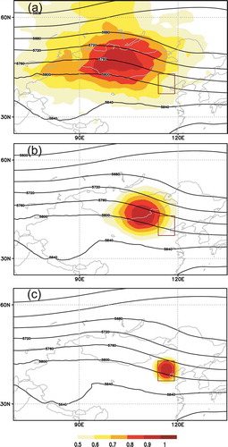
The 3-month calculations cover the whole summer period (June, July, and August) in 2017. Instead of using a constant guess analysis error matrix in Z2016, the analysis error matrix is approximated by the ensemble spreads at the sensitivity analysis time, which is expected to capture some flow-dependent structures of the error covariance. Figure 1 shows the 3-month averaged sensitivity regions to improve forecast over Beijing with different lead times. It is seen that Beijing is in front of the pressure ridge at 500 hPa. The sensitivity region with maximum total energy is located within the verification region at 0-day lead time, and moves to upstream region with longer lead times. The main signal at 2-day lead times is located in Mongolia area where is less of conventional meteorological observations. It indicates more remote data like satellite radiances might be help to improve 2-day wind and temperature forecasts over Beijing region. And an advanced data assimilation system that can spread observation information from China to improve analysis over Mongolia area might also be helpful.

Figure 1. Three-month averaged sensitivity regions (shaded) to improve forecasts over Beijing with different lead times, (a) 2 days, (b) 1 day, and (c) 0 day. Three-month averaged ensemble mean geopotential height at 500 hPa is denoted by black contours. The verification region is shown by the rectangular. The signal is rescaled with the maximum value of the total energy in the domain.

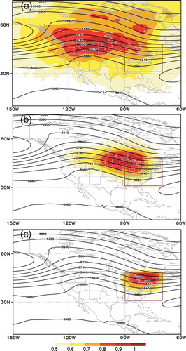
Figure 2 shows the 3-month averaged sensitivity regions to improve forecast over eastern regions of U.S.A with different lead times. It is seen that the eastern regions of the U.S.A is dominated by a 500 hPa trough. The sensitivity region with maximum total energy is located within the verification region at 0-day lead time, and moves to northwestern upstream region with longer lead times. The main signals are located over the North American that are rich of conventional observations, which indicates that a regional forecasting system has a good chance to make accurate forecasts over eastern regions of U.S.A up to 2 days in summer when those data are well quality screened and assimilated.

Figure 2. Three-month averaged sensitivity regions (shaded) to improve forecasts over eastern regions of U.S.A with different lead times, (a) 2 days, (b) 1 day, and (c) 0 day. Three-month averaged ensemble mean geopotential height at 500 hPa is denoted by black contours. The verification region is shown by the rectangular. The signal is rescaled with the maximum value of the total energy in the domain.

4. Summary

Ensemble-based sensitivity analysis methods are computationally efficient provided an ensemble of forecast are already available. The ET method proposed by Bishop and Toth (1999, hereafter BT1999), and a variation ET-based sensitivity (ETS) method (Zhang et al. 2016) have been used to specify sensitive area for adaptive observations. The ETS method increases computation efficiency by calculating the gradient of forecast error variance reduction in terms of analysis error variance reduction that only requires one calculation of the ensemble transformation matrix.

In this paper, it is noted that the solution of the ensemble transformation matrix in the ET and ETS methods is not unique. A general mathematical formulation for the ensemble transformation matrix is derived and then a general mathematical formulation of the ETS is described. It is proved that the ET formulation in BT199 and ETS formulation in Z2016 are special implementations of the general ET and ETS formulations.

Under some conditions, it is shown that the ETS signal is proportional to amplitude of analysis error variance. In other words, ETS intends to identify region of larger analysis error variance as data sensitive area. This feature is physically meaningful because that targeted observations should be placed in regions where the analysis errors have room to be reduced. The larger analysis errors in regions are, the more room to reduce the error. Another more efficient implementation of the ETS formulation, which inherits the above feature and avoids calculating inverse process of some matrices, is proposed. In the practical implementation of this efficient ETS, the flow-dependent ensemble spread is used to represent the analysis error variance, whereas Z2016 used constant analysis error variances that does not vary with locations.

The three-month averaged sensitivity regions for improving forecasts during summer 2017 over Bejing, China and eastern regions of U.S with forecasting lead times up to two days show reasonable sensitivity regions that locate in upstream of the verification regions. Moreover, the general formulation provides an opportunity to investigate the uncertainty of the different ET and ETS implementations on sensitivity areas identified for adaptive observations and/or observation network optimization. This can be a subject of future studies.

Disclosure statement

No potential conflict of interest was reported by the authors.

References

- Ancell, B., and G. J. Hakim. 2007. “Comparing Adjoint- and Ensemble-Sensitivity Analysis with Applications to Observation Targeting.” Monthly Weather Review 135: 4117–4134. doi:10.1175/2007MWR1904.1.
- Bishop, C. H., B. J. Etherton, and S. J. Majumdar. 2001. “Adaptive Sampling with the Ensemble Transform Kalman Filter. Part I: Theoretical Aspects.” Monthly Weather Review 129: 420–436. doi:10.1175/1520-0493(2001)129<0420:ASWTET>2.0.CO;2.
- Bishop, C. H., and Z. Toth. 1999. “Ensemble Transformation and Adaptive Observations.” Journal of the Atmospheric Sciences 56: 1748–1765. doi:10.1175/1520-0469(1999)056<1748:ETAAO>2.0.CO;2.
- Buizza, R., and A. Montani. 1999. “Targeted Observations Using Singular Vectors.” Journal of the Atmospheric Sciences 56: 2965–2985. doi:10.1175/1520-0469(1999)056<2965:TOUSV>2.0.CO;2.
- Chang, E. K. M., M. H. Zheng, and K. Raeder. 2013. “Medium-Range Ensemble Sensitivity Analysis of Two Extreme Pacific Extratropical Cyclones.” Monthly Weather Review 141: 211–231. doi:10.1175/MWR-D-11-00304.1.
- Ito, K., and -C.-C. Wu. 2013. “Typhoon-Position-Oriented Sensitivity Analysis. Part I: Theory and Verification.” Journal of the Atmospheric Sciences 70: 2525–2546. doi:10.1175/JAS-D-12-0301.1.
- Majumdar, S. J., C. H. Bishop, B. J. Etherton, and Z. Toth. 2002. “Adaptive Sampling with the Ensemble Transform Kalman Filter. Part II: Field Program Implementation.” Monthly Weather Review 130: 1356–1369. doi:10.1175/1520-0493(2002)130<1356:ASWTET>2.0.CO;2.
- Mu, M., F. F. Zhou, and H. L. Wang. 2009. “A Method for Identifying the Sensitive Areas in Targeted Observations for Tropical Cyclone Prediction: Conditional Nonlinear Optimal Perturbation.” Monthly Weather Review 137: 1623–1639. doi:10.1175/2008MWR2640.1.
- Palmer, T. N., R. Gelaro, J. Barkmeijer, and R. Buizza. 1998. “Singular Vectors, Metrics, and Adaptive Observations.” Journal of the Atmospheric Sciences 55: 633–653. doi:10.1175/1520-0469(1998)055<0633:SVMAAO>2.0.CO;2.
- Wang, H. L., M. Mu, and X. Y. Huang. 2011. “Application of Conditional Non-Linear Optimal Perturbations to Tropical Cyclone Adaptive Observation Using the Weather Research Forecasting (WRF) Model.” Tellus A 63: 939–957. doi:10.1111/j.1600-0870.2011.00536.x.
- Xie, B. G., F. Q. Zhang, Q. H. Zhang, J. Poterjoy, and Y. H. Weng. 2013. “Observing Strategy and Observation Targeting for Tropical Cyclones Using Ensemble-Based Sensitivity Analysis and Data Assimilation.” Monthly Weather Review 141: 1437–1453. doi:10.1175/MWR-D-12-00188.1.
- Yu. H., H. Wang, Z. Meng, M. Mu, X. Huang, and X. Zhang. 2017. “A WRF-Based Tool for Forecast Sensitivity to the Initial Perturbation: The Conditional Nonlinear Optimal Perturbations versus the First Singular Vector Method and Comparison to MM5”. Journal of Atmospheric and Oceanic Technology 34: 187–206. doi:10.1175/JTECH-D-15-0183.1.
- Zhang, Y., Y. Xie, H. Wang, D. Chen, and Z. Toth. 2016. “Ensemble Transformation Sensitivity Method for Adaptive Observations.” Advances in Atmospheric Sciences 33: 10–20. doi:10.1007/s00376-015-5031-9.