Simulated and projected relationship between the East Asian winter monsoon and winter Arctic Oscillation in CMIP5 models

ABSTRACT

Interdecadal change in the relationship between the East Asian winter monsoon (EAWM) and the Arctic Oscillation (AO) has been documented by many studies. This study, utilizing the model outputs from phase 5 of the Coupled Model Intercomparison Project (CMIP5), evaluates the ability of the coupled models in CMIP5 to capture the intensified relationship between the EAWM and winter AO since the 1980s, and further projects the evolution of the EAWM–AO relationship during the 21st century. It is found that the observed evolution of the EAWM–AO relationship can be reproduced well by some coupled models (e.g., GFDL-ESM2M, GISS-E2-H, and MPI-ESM-MR). The coupled models’ simulations indicate that the impact of winter AO on the EAWM-related circulation and East Asian winter temperature has strengthened since the 1980s. Such interdecadal change in the EAWM–AO relationship is attributed to the intensified propagation of stationary planetary waves associated with winter AO. Projections under the RCP4.5 and RCP8.5 scenarios suggest that the EAWM–AO relationship is significant before the 2030s and after the early 2070s, and insignificant during the 2060s, but uncertain from the 2030s to the 2050s.

摘要

观测资料显示，东亚冬季风与同期AO的关系在20世纪80年代发生年代际增强。通过考察CMIP5模式对这一现象的模拟情况，发现GFDL-ESM2M、GISS-E2-H和MPI-ESM-MR这3个模式能够再现EAWM-AO关系的年代际增强。进一步考察这3个模式的集合平均结果（MME）发现，冬季AO对EAWM环流系统以及东亚气温的影响均发生明显的年代际变化。通过考察MME模拟的EP通量结果发现，自20世纪80年代开始，在对流层从高纬度地区传播到副热带地区的EP通量异常明显增强，这是MME模拟结果中EAWM-AO关系发生年代际增强的主要原因。

KEYWORDS:

• East Asian winter monsoon (EAWM)
• winter Arctic Oscillation (AO)
• CMIP5
• interdecadal change

1. Introduction

The East Asian winter monsoon (EAWM) is one of the most active large-scale atmospheric circulation systems over the Northern Hemisphere and shows intraseasonal, interannual, and decadal variations (Ding et al. 2014; Wang and Lu 2017). Concurrent with a stronger-than-normal EAWM, the Siberian high and Aleutian low are strikingly reinforced, which could lead to intensely northerly wind along the coast of East Asia. Meanwhile, the East Asian trough and the meridional shear of the East Asian jet stream (EAJS) are strengthened as well (He and Wang 2012).

Previous investigations have indicated that the intensity of the EAWM is related to many factors, such as the Arctic Oscillation (AO), El Niño–Southern Oscillation, Hadley circulation, Eurasian snow cover, and Arctic sea ice (Webster and Yang 1992; Zhang, Sumi, and Kimoto 1996; Watanabe and Nitta 1999; Chen, Graf, and Huang 2000; Zhou and Wang 2008; Li and Wang 2013; Wang and Liu 2016; He et al. 2017). Among these factors, the AO, as the dominant mode of the extratropical atmospheric circulation over the Northern Hemisphere, has been found to exert great effects on the East Asian climate and the EAWM (Thompson and Wallace 1998; Zhou 2017). According to Gong, Wang, and Zhu (2001), the winter AO may affect the EAWM by modulating the Siberian high. In contrast, Wu and Wang (2002) emphasized the direct impact of winter AO on the EAWM-related atmospheric circulation.

Recently, it has been found that the EAWM–AO relationship is unstable. Since the 1980s, the EAWM–AO relationship is noticeably enhanced (Li, Wang, and Gao 2014). Such strengthening may be caused by the diminished autumn Arctic sea-ice cover, which could trigger the westward intrusion of the EAJS from the Northwest Pacific toward East Asia. Lu, Zhou, and Ding (2016) also found that, after 2000, the stratospheric polar vortex disturbances increase and the Northern Hemisphere Annular Mode is mainly in negative phase. Therefore, the Urals blocking high and East Asian trough are more active after 2000, which lead to enhanced cold air activities in eastern and northern China.

Given the important influence of AO on the EAWM and the unstable relationship between the EAWM and AO, it is necessary to gain more insights into the future changes of the EAWM, AO, and EAWM–AO relationship. There have been numerous projections concerning the future evolution of the EAWM (Hu, Bengtsson, and Arpe 2000; Jiang and Tian 2013) and AO (Miller, Schmidt, and Shindell 2006; Gillett and Fyfe 2013; Sun and Ahn 2015; Zhu and Wang 2016). However, few studies have discussed the future change of the EAWM–AO relationship. To what extent can state-of-the-art coupled models simulate the interdecadal change of the EAWM–AO relationship? How will the EAWM–AO relationship evolve during the 21st century? These issues are analyzed in this article using historical simulations and future projections under different Representative Concentration Pathway (RCP) scenarios in phase 5 of the Coupled Model Intercomparison Project (CMIP5).

2. Data and methods

The historical simulations and future projections under the RCP4.5 and RCP8.5 scenarios from 33 CMIP5 models (Taylor, Stouffer, and Meehl 2012) are offered by the PCMDI (Program for Climate Model Diagnosis and Intercomparison). Here, we only analyze the first realization (r1i1p1) of each individual model. The reanalysis datasets from the National Centers for Environmental Prediction–National Center for Atmospheric Research (NCEP–NCAR) (Kalnay et al. 1996) are used to compare with historical simulations.

There are many indices to measure the EAWM. Wang and Chen (2010b) classified these indices into four categories. They also found that some EAWM indices are not suitable for describing the EAWM–AO relationship. Since Li, Wang, and Gao (2014) identified the strengthened EAWM–AO relationship around the 1980s in observations, we define the EAWM index as in their study. We calculate the EAWM index as the average of three different EAWM indices. The first index is defined as the area-averaged (25°–50°N, 115°–145°E) wind speed at 850 hPa (Wang and Jiang 2004). The second index is defined as the area-averaged (25°–45°N, 110°–145°E) geopotential height at 500 hPa (Wang and He 2012). The third index is defined as the zonal wind shear at 200 hPa (Li and Yang 2010), which is calculated as area-averaged (30°–35°N, 90°–160°E) 200-hPa zonal wind minus half of the area-averaged (50°–60°N, 70°–170°E) 200-hPa zonal wind and half of the area-averaged (5°S–10°N, 90°–160°E) 200-hPa zonal wind. Before computing the average of these three indices, all three indices are linearly detrended and normalized. The AO index is defined as the time series of the leading empirical orthogonal function mode of sea level pressure (SLP) anomalies northward of 20°N. The EAJS index is calculated as the area-averaged (30°–35°N, 130°–160°E) zonal wind at 200 hPa (Yang, Lau, and Kim 2002).

We use Eliassen–Palm (EP) flux to diagnose the interaction between waves and mean flow (Andrews, Holton, and Leovy 1987). The following is the meridional and vertical constituents of the EP flux:

(1)

(2)

Here, is the radius of Earth, is the latitude, and are the zonal and meridional wind, is the Coriolis parameter, is the potential temperature, is the pressure, and . The primes and overbars represent zonal deviations and averages, respectively. In this study, the vectors are multiplied by , and the vertical constituent times 125.

The selected periods for historical simulations and future projections are the winters of 1950–2003 and 2006–99, respectively. Here, as an example, the winter of 1950 stands for the December of 1950 and the January and February of 1951. All data and indices are linearly detrended prior to examination.

3. Results

3.1. The EAWM–AO relationship in the historical simulations

Figure 1(a) shows the 21-yr sliding correlation coefficients between the EAWM index and the negative AO (−AO) index in the NCEP–NCAR reanalysis datasets. Apparently, the EAWM–AO relationship is strikingly strengthened since the 1980s, which is consistent with the results of Li, Wang, and Gao (2014). Then, the entire period (1950–2003) is divided into two sub-periods: 1950–1970 and 1980–2003. As displayed in Table 1, for the entire period, the correlation coefficient of the observed EAWM–AO relationship is 0.416 (above the 90% confidence level). Meanwhile, the insignificant correlation of 0.341 during 1950–70 increases to a strong stage of 0.495 during 1980–2003.

Table 1. Correlation coefficients between the EAWM index and the −AO index during the winters of 1950–70, 1980–2003, and 1950–2003 for the NCEP–NCAR reanalysis data and each CMIP5 model. The bold values are significant at the 90% confidence level according to the student’s t-test. The models reproducing the strengthened EAWM–AO relationship since the 1980s are in bold.

	1950–70	1980–2003	1950–2003
Obs.	0.341	0.495	0.416
ACCESS1.3	0.769	0.860	0.807
BCC-CSM1.1	0.378	0.480	0.425
BCC-CSM1.1(m)	0.728	0.834	0.793
BNU-ESM	0.681	0.511	0.621
CanESM2	0.733	0.562	0.643
CESM1(BGC)	0.443	0.266	0.379
CESM1(CAM5)	0.162	0.333	0.343
CMCC-CM	0.712	0.758	0.702
CMCC-CMS	–0.138	0.111	0.028
CNRM-CM5	0.378	0.817	0.625
FGOALS-s2	0.374	0.446	0.386
FGOALS-g2	0.379	0.631	0.521
GFDL-CM3	0.401	0.755	0.533
GFDL-ESM2G	0.738	0.686	0.653
GFDL-ESM2M	0.105	0.556	0.453
GISS-E2-H	0.316	0.369	0.372
GISS-E2-R	0.584	0.327	0.375
HadCM3	0.739	0.826	0.769
HadGEM2-AO	0.601	0.424	0.478
HadGEM2-CC	0.451	0.651	0.597
HadGEM2-ES	–0.361	0.067	–0.125
INM-CM4	0.708	0.707	0.713
IPSL-CM5A-LR	0.498	0.620	0.566
IPSL-CM5A-MR	0.599	0.723	0.640
IPSL-CM5B-LR	0.200	0.069	0.179
MIROC4h	0.603	–0.062	0.254
MIROC5	0.156	–0.164	–0.065
MIROC-ESM	0.659	0.474	0.591
MIROC-ESM-CHEM	0.535	0.491	0.526
MPI-ESM-MR	0.342	0.363	0.290
MRI-CGCM3	0.385	0.180	0.310
NorESM1-M	0.632	0.699	0.665
NorESM1-ME	0.661	0.372	0.524

Figure 1. The 21-yr sliding correlation coefficients between the EAWM index and the −AO index during the winters of 1950–2003 for the (a) NCEP–NCAR reanalysis data and (b) MME. The 21-yr sliding correlation coefficients between the EAJS index and the −AO index during the winters of 1950–2003 for the (c) NCEP–NCAR reanalysis data and (d) MME. The horizontal long (short) dashed line indicates the 90% (95%) confidence level according to the student’s t-test. The shading indicates one intermodel standard deviation departure from the MME mean.

But can the latest CMIP5 models reproduce the interdecadal change of the EAWM–AO relationship? To answer this question, we calculate the EAWM–AO correlation coefficients in each individual model. As shown in Table 1, almost all the CMIP5 models can replicate the statistically significant EAWM–AO relationship during 1950–2003, except for CMCC-CMS, HadGEM2-ES, IPSL-CM5B-LR, and MIROC5. Meanwhile, there are three models — GFDL-ESM2M, GISS-E2-H, and MPI-ESM-MR – that can capture well the interdecadal shift of the EAWM–AO relationship around the 1980s. Clearly, most of the CMIP5 models fail to reproduce the intensified EAWM–AO relationship, which may be attributable to the biases of CMIP5 models in simulating the basic features of the EAWM and AO. As indicated in previous studies, most of the CMIP5 models overestimate the intensity of the Pacific center in the wintertime AO pattern (Gong et al. 2017) and have lower capability in simulating the interannual variability of the EAWM system (Gong et al. 2014). With these biases, the skill of CMIP5 models in reproducing the interdecadal shift of the EAWM–AO relationship may be limited. Considering the good ability of these three models to capture the variation in the EAWM–AO relationship, we calculate the 21-yr sliding correlation coefficients between the EAWM index and the −AO index using the multi-model ensemble (MME) mean results of these three models. Results of the MME (Figure 1(b)) show that the EAWM–AO relationship is generally strengthened since the 1980s. Although the temporal evolution of the EAWM–AO relationship in the MME shows biases to the individual models (Figure 1(b): shading), the results of both individual models and the MME exhibit continuous intensification of the EAWM–AO relationship. It should be noted that, if we use the 95% confidence level for the model selection, six models — BCC-CSM1.1, CNRM-CM5, FGOALS-s2, FGOALS-g2, GFDL-CM3, and GFDL-ESM2M — will be identified, the ensemble mean of which can also reproduce the observed intensified EAWM–AO relationship (figures not shown). Given that the results of the MME match better with the observation, we mainly examine the simulations of the MME for the following analysis.

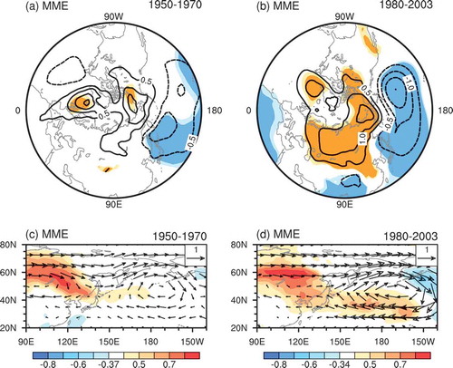
Corresponding to the interdecadal shift of the EAWM–AO relationship in the MME, there are notable changes in the simulated EAWM/AO-related atmospheric circulation from 1950–70 to 1980–2003. Firstly, we regress the SLP upon the EAWM index. During 1950–70 (Figure 2(a)), significantly negative SLP anomalies are primarily located over East Asia and the Northwest Pacific, while the positive SLP anomalies over the Arctic are weak and barely significant. During 1980–2003 (Figure 2(b)), the positive center over the Arctic is markedly reinforced, rendering an AO-like seesaw pattern over the mid and high latitudes. These features suggest that the EAWM shows a stronger linkage with the winter AO during the latter period. Further investigations of the AO-related atmospheric circulation also support this conclusion. Since the 1980s, the AO-related southerly wind anomalies near the coast of East Asia strikingly intensify (Figure 2(d) versus Figure 2(c): vectors), accompanied by more southeastward invasion of warm anomalies (Figure 2(d) versus Figure 2(c): shading).

Figure 2. Regression maps of SLP anomalies (units: hPa) upon the EAWM index during (a) 1950–70 and (b) 1980–2003. Light (dark) shading indicates the 90% (95%) confidence level according to the student’s t-test. Correlation coefficients (shading) of surface air temperature anomalies (units: °C) and regression coefficients (vectors) of 700-hPa wind anomalies (units: m s⁻¹) upon the winter AO index during (c) 1950–70 and (d) 1980–2003.

According to Li, Wang, and Gao (2014), the EAJS plays a crucial role in linking the EAWM and winter AO since the 1980s, which is reflected by the strikingly enhanced EAJS–AO relationship in reanalysis datasets (Figure 1(c)) and the MME (Figure 1(d)). To further examine such a role of the EAJS in the MME, we inspect the regression maps of the SLP upon the EAJS index. During 1950–70 (Figure 3(a)), two significant negative centers are located over the North Pacific and Northwest Atlantic, with tenuous signals over the Arctic. During 1980–2003 (Figure 3(b)), the positive center over the Arctic strengthens and becomes statistically significant, inducing a notable Arctic–Pacific dipole. These characteristics imply an enhanced EAJS–AO relationship in the latter period.

Figure 3. Regression maps of SLP anomalies (units: hPa) upon the EAJS index during the winters of (a) 1950–70 and (b) 1980–2003. Light (dark) shading indicates the 90% (95%) confidence level according to the student’s t test. Regression maps of zonally averaged zonal wind anomalies (units: m s⁻¹) upon the winter AO index during (c) 1950–70 and (d) 1980–2003. Light (dark) shading indicates the 90% (95%) confidence level according to the Student’s t-test. Differences of zonally averaged zonal wind (blue contours; units: m s⁻¹), EP flux cross sections (vectors; units: 10⁸ m² s⁻²), and its divergence (red contours; units: m s⁻¹ d⁻¹) between high (≥ 0.5 standard deviation) and low (≤ −0.5 standard deviation) winter AO index during (e) 1950–70 and (f) 1980–2003. The shading indicates zonally averaged zonal wind significant at the 90% confidence level according to the student’s t-test.

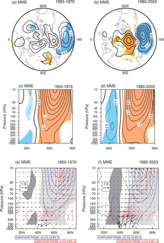
To verify the changes in the AO-related atmospheric circulation in the MME, the zonally averaged zonal wind is regressed. During 1950–70 (Figure 3(c)), the negative anomalies at the midlatitudes are weak and mainly confined to the lower troposphere. During 1980–2003 (Figure 3(d)), the negative anomalies at the midlatitudes are strikingly intensified, with more significant anomalies extending upward to the stratosphere. The vertical structure resembles the classical structure of the AO. It implies that the winter AO shows a stronger connection with the EAJS in the latter period, which could bond the linkage between the EAWM and winter AO (Li, Wang, and Gao 2014).

Given that stationary planetary waves play an important role in the connection between the EAWM and AO (Chen, Yang, and Huang 2005; Wang and Chen 2010a), we further investigate the changes of stationary planetary waves associated with the winter AO by analyzing the EP flux in the MME, the aim being to explain the possible mechanism underlying the intensified EAWM–AO relationship at the interdecadal scale. During 1980–2003, apparent anomalous EP flux divergence appears in the troposphere and stratosphere near 60°N (Figure 3(f): red contours), which implies that the westerly zonal-mean flow accelerates there (Andrews, Holton, and Leovy 1987). Subsequently, the polar night jet strengthens significantly (Figure 3(f): blue contours around 60°N). Another notable feature is the apparent low-level waveguide propagating from the high latitudes equatorward to the subtropics, leading to significant anomalies of the subtropical jet stream (Figure 3(f): blue contours around 30°N). Thus, the propagation of stationary planetary waves favors the close connection between the winter AO and the EAJS/EAWM during 1980–2003. During 1950–70 (Figure 3(e)), although the anomalous EP flux divergence remains in the troposphere near 60°N, the equatorward propagating EP flux is relatively weak. Therefore, the linkage between the winter AO and the EAJS/EAWM during 1950–70 is weaker than that during 1980–2003.

3.2. Projected EAWM–AO relationship under the RCP4.5 and RCP8.5 scenarios

In view of the reasonable reproducibility in the MME, another question we want to address is how the EAWM–AO relationship may evolve during the 21st century. Using the future projections of the MME, the projected EAWM–AO relationship under the RCP4.5 and RCP8.5 scenarios tends to remain unstable (Figure 4). Before the 2030s, the EAWM–AO relationship is statistically significant under the RCP4.5 and RCP8.5 scenarios, and the EAWM–AO correlation coefficients are around 0.6. During the 2030s, the EAWM–AO correlation coefficients reduce to 0.3 (below the 90% confidence level) under the RCP4.5 scenario. By contrast, the EAWM is still closely related to the simultaneous AO during the 2030s under the RCP8.5 scenario, and the EAWM–AO correlation coefficients remain around 0.6. During the 2040s and 2050s, the EAWM–AO correlation coefficients are projected to gradually recover to 0.6 under the RCP4.5 scenario. However, the EAWM–AO relationship under the RCP8.5 scenario experiences a rapid weakening in the early 2040s, and remains around the 90% confidence level during the 2040s and 2050s. During the 2060s, the EAWM–AO relationship becomes insignificant again under the RCP4.5 scenario, while the relationship remains relatively weak under the RCP8.5 scenario. Finally, the EAWM–AO correlation coefficients return back to 0.7 after the early 2070s under both RCP4.5 and RCP8.5 scenarios. Therefore, projections under both the RCP4.5 and RCP8.5 scenarios suggest a significant EAWM–AO relationship before the 2030s and after the early 2070s, and an insignificant relationship during the 2060s. However, from the 2030s to the 2050s, the projected EAWM–AO relationship under the RCP4.5 scenario is contrary to that projected under the RCP8.5 scenario, which implies uncertainty in the EAWM–AO relationship during the mid-term of the 21st century.

Figure 4. The 21-yr sliding correlation coefficients between the EAWM index and the −AO index during the winters of 2006–99 for the MME under the (a) RCP4.5 scenario and (b) RCP8.5 scenario. The horizontal long (short) dashed line indicates the 90% (95%) confidence level according to the student’s t-test. The shading indicates one intermodel standard deviation departure from the MME mean.

4. Summary and discussion

This study investigates how the latest CMIP5 models simulate the interdecadal change of the EAWM–AO relationship and how this relationship may evolve during the 21st century.

Comparisons between 1950–70 and 1980–2003 indicate that there are three models — GFDL-ESM2M, GISS-E2-H, and MPI-ESM-MR — that can capture well the interdecadal shift of the EAWM–AO relationship around the 1980s. The simulated atmospheric circulation of the MME also supports such interdecadal change. Compared with the former period, the EAWM-associated SLP anomalies in the latter period are characterized by an AO-like pattern. Concurrent with a positive phase of winter AO, the anomalous southerly wind near the coast of East Asia clearly reinforces during 1980–2003, accompanied by more southeastward invasion of warm anomalies. These characteristics suggest an enhanced EAWM–AO relationship since the 1980s.

The historical simulations of the MME also demonstrate the crucial role of the EAJS in linking the EAWM and winter AO since the 1980s. During 1950–70, the AO-related zonally averaged zonal wind anomalies at the midlatitudes are weak and mainly confined to the lower troposphere. During 1980–2003, the anomalies at the midlatitudes are strikingly intensified, rendering a classical structure of the AO. Therefore, the winter AO shows a stronger connection with the EAJS/EAWM in the latter period. To explain the possible mechanism underlying the strengthened EAWM–AO relationship, we further gain an insight into the changes of stationary planetary waves associated with the winter AO in the MME. During 1980–2003, apparent low-level EP flux propagates from the high latitudes equatorward to the subtropics, leading to significant anomalies of the subtropical jet stream. This accounts for the close connection between the winter AO and the EAJS/EAWM in the latter period. During 1950–70, the equatorward propagating EP flux is relatively weak. Therefore, the linkage between the winter AO and the EAJS/EAWM during 1950–70 is weaker than that during 1980–2003.

Finally, we discuss the projected EAWM–AO relationship in the MME. Projections under both the RCP4.5 and RCP8.5 scenarios suggest a significant EAWM–AO relationship before the 2030s and after the early 2070s, and an insignificant one during the 2060s. However, from the 2030s to the 2050s, the projected EAWM–AO relationship under the RCP4.5 scenario is contrary to that projected under the RCP8.5 scenario, which implies uncertainty in the EAWM–AO relationship during the mid-term of the 21st century.

Disclosure statement

No potential conflict of interest was reported by the authors.

Additional information

Funding

This work was supported by the National Natural Science Foundation of China [grants numbers 41505073 and 41605059] and the Young Talent Support Program by the China Association for Science and Technology [grant number 2016QNRC001].

References

- Andrews, D. G., J. R. Holton, and C. B. Leovy. 1987. Middle Atmosphere Dynamics. San Diego, California: Academic Press.
- Chen, W., S. Yang, and R. H. Huang. 2005. “Relationship between Stationary Planetary Wave Activity and the East Asian Winter Monsoon.” Journal of Geophysical Research: Atmospheres 110 (D14). doi:10.1029/2004JD005669.
- Chen, W. H. F. Graf, and R. Huang. 2000. “The Interannual Variability of East Asian Winter Monsoon and Its Relation to the Summer Monsoon.” Advances in Atmospheric Sciences 17 (1): 48–60. doi: 10.1007/s00376-000-0042-5.
- Ding, Y. H., Y. J. Liu, S. J. Liang, X. Q. Ma, Y. X. Zhang, D. Si, P. Liang, Y. F. Song, and J. Zhang. 2014. “Interdecadal Variability of the East Asian Winter Monsoon and Its Possible Links to Global Climate Change.” Journal of Meteorological Research 28 (5): 693–713. doi:10.1007/s13351-014-4046-y.
- Gillett, N. P., and J. C. Fyfe. 2013. “Annular Mode Changes in the CMIP5 Simulations.” Geophysical Research Letters 40 (6): 1189–1193. doi:10.1002/grl.50249.
- Gong, D. Y., S. W. Wang, and J. H. Zhu. 2001. “East Asian Winter Monsoon and Arctic Oscillation.” Geophysical Research Letters 28 (10): 2073–2076. doi:10.1029/2000GL012311.
- Gong, H. N., L. Wang, W. Chen, R. G. Wu, K. Wei, and X. F. Cui. 2014. “The Climatology and Interannual Variability of the East Asian Winter Monsoon in CMIP5 Models.” Journal of Climate 27 (4): 1659–1678. doi:10.1175/JCLI-D-13-00039.1.
- Gong, H. N., L. Wang, W. Chen, X. L. Chen, and D. Nath. 2017. “Biases of the Wintertime Arctic Oscillation in CMIP5 Models.” Environmental Research Letters 12 (1). doi:10.1088/1748-9326/12/1/014001.
- He, S. P., and H. J. Wang. 2012. “An Integrated East Asian Winter Monsoon Index and Its Interannual Variability (In Chinese).” Chinese Journal of Atmospheric Sciences 36 (3): 523–538.
- He, S. P., Y. Q. Gao, F. Li, H. J. Wang, and Y. C. He. 2017. “Impact of Arctic Oscillation on the East Asian Climate: A Review.” Earth-Science Reviews 164: 48–62. doi:10.1016/j.earscirev.2016.10.014.
- Hu, Z. Z., L. Bengtsson, and K. Arpe. 2000. “Impact of Global Warming on the Asian Winter Monsoon in a Coupled GCM.” Journal of Geophysical Research: Atmospheres 105 (D4): 4607–4624. doi:10.1029/1999JD901031.
- Jiang, D. B., and Z. P. Tian. 2013. “East Asian Monsoon Change for the 21st Century: Results of CMIP3 and CMIP5 Models.” Chinese Science Bulletin 58 (12): 1427–1435. doi:10.1007/s11434-012-5533-0.
- Kalnay, E., M. Kanamitsu, R. Kistler, W. Collins, D. Deaven, L. Gandin, M. Iredell, et al. 1996. “The NCEP/NCAR 40-Year Reanalysis Project.” Bulletin of the American Meteorological Society 77 (3): 437–471. doi:10.1175/1520-0477(1996)077<0437:TNYRP>2.0.CO;2.
- Li, F., and H. J. Wang. 2013. “Relationship between Bering Sea Ice Cover and East Asian Winter Monsoon Year-To-Year Variations.” Advances in Atmospheric Sciences 30 (1): 48–56. doi:10.1007/s00376-012-2071-2.
- Li, F., H. J. Wang, and Y. Q. Gao. 2014. “On the Strengthened Relationship between the East Asian Winter Monsoon and Arctic Oscillation: A Comparison of 1950–70 and 1983–2012.” Journal of Climate 27 (13): 5075–5091. doi:10.1175/JCLI-D-13-00335.1.
- Li, Y. Q., and S. Yang. 2010. “A Dynamical Index for the East Asian Winter Monsoon.” Journal of Climate 23 (15): 4255–4262. doi:10.1175/2010JCLI3375.1.
- Lu, C. H., B. T. Zhou, and Y. H. Ding. 2016. “Decadal Variation of the Northern Hemisphere Annular Mode and Its Influence on the East Asian Trough.” Journal of Meteorological Research 30 (4): 584–597. doi:10.1007/s13351-016-5105-3.
- Miller, R. L., G. A. Schmidt, and D. T. Shindell. 2006. “Forced Annular Variations in the 20th Century Intergovernmental Panel on Climate Change Fourth Assessment Report Models.” Journal of Geophysical Research-Atmospheres 111 (D18). doi:10.1029/2005JD006323.
- Sun, J. Q., and J. B. Ahn. 2015. “Dynamical Seasonal Predictability of the Arctic Oscillation Using a CGCM.” International Journal of Climatology 35 (7): 1342–1353. doi:10.1002/joc.4060.
- Taylor, K. E., R. J. Stouffer, and G. A. Meehl. 2012. “An Overview of CMIP5 and the Experiment Design.” Bulletin of the American Meteorological Society 93 (4): 485–498. doi:10.1175/BAMS-D-11-00094.1.
- Thompson, D. W. J., and J. M. Wallace. 1998. “The Arctic Oscillation Signature in the Wintertime Geopotential Height and Temperature Fields.” Geophysical Research Letters 25 (9): 1297–1300. doi:10.1029/98GL00950.
- Wang, H. J., and D. B. Jiang. 2004. “A New East Asian Winter Monsoon Intensity Index and Atmospheric Circulation Comparison between Strong and Weak Composite (In Chinese).” Quaternary Sciences 24 (1): 19–27.
- Wang, H. J., and S. P. He. 2012. “Weakening Relationship between East Asian Winter Monsoon and ENSO after Mid-1970s.” Chinese Science Bulletin 57 (27): 3535–3540. doi:10.1007/s11434-012-5285-x.
- Wang, L., and M. M. Lu. 2017. “The East Asian Winter Monsoon.” In The Global Monsoon System: Research and Forecast (3rd ed.), 51–61. Singapore: World Scientific.
- Wang, L., and W. Chen. 2010a. “Downward Arctic Oscillation Signal Associated with Moderate Weak Stratospheric Polar Vortex and the Cold December 2009.” Geophysical Research Letters 37. doi:10.1029/2010GL042659.
- Wang, L., and W. Chen. 2010b. “How Well Do Existing Indices Measure the Strength of the East Asian Winter Monsoon?” Advances in Atmospheric Sciences 27 (4): 855–870. doi:10.1007/s00376-009-9094-3.
- Wang, S. Y., and J. P. Liu. 2016. “Delving into the Relationship between Autumn Arctic Sea Ice and Central-Eastern Eurasian Winter Climate.” Atmospheric and Oceanic Science Letters 9 (5): 366–374. doi:10.1080/16742834.2016.1207482.
- Watanabe, M., and T. Nitta. 1999. “Decadal Changes in the Atmospheric Circulation and Associated Surface Climate Variations in the Northern Hemisphere Winter.” Journal of Climate 12 (2): 494–510. doi:10.1175/1520-0442(1999)012<0494:DCITAC>2.0.CO;2.
- Webster, P. J., and S. Yang. 1992. “Monsoon and ENSO: Selectively Interactive Systems.” Quarterly Journal of the Royal Meteorological Society 118 (507): 877–926. doi:10.1002/(ISSN)1477-870X.
- Wu, B. Y., and J. Wang. 2002. “Winter Arctic Oscillation, Siberian High and East Asian Winter Monsoon.” Geophysical Research Letters 29 (19). doi:10.1029/2002GL015373.
- Yang, S., K. M. Lau, and K. M. Kim. 2002. “Variations of the East Asian Jet Stream and Asian-Pacific-American Winter Climate Anomalies.” Journal of Climate 15 (3): 306–325. doi:10.1175/1520-0442(2002)015<0306:VOTEAJ>2.0.CO;2.
- Zhang, R. H., A. Sumi, and M. Kimoto. 1996. “Impact of El Niño on the East Asian Monsoon: A Diagnostic Study of the ‘86/87 and ‘91/92 Events.” Journal of the Meteorological Society of Japan 74 (1): 49–62. doi:10.2151/jmsj1965.74.1_49.
- Zhou, B. T., and H. J. Wang. 2008. “Interdecadal Change in the Connection between Hadley Circulation and Winter Temperature in East Asia.” Advances in Atmospheric Sciences 25 (1): 24–30. doi:10.1007/s00376-008-0024-6.
- Zhou, W. 2017. “Impact of Arctic Amplification on East Asian Winter Climate.” Atmospheric and Oceanic Science Letters 10 (5): 385–388. doi:10.1080/16742834.2017.1350093.
- Zhu, Y. L., and T. Wang. 2016. “The Relationship between the Arctic Oscillation and ENSO as Simulated by CCSM4.” Atmospheric and Oceanic Science Letters 9 (3): 198–203. doi:10.1080/16742834.2016.1149287.