A new global ocean hydrographic climatology

ABSTRACT

This report describes the main features of the recently published World Ocean Experiment–Argo Global Hydrographic Climatology. This climatology is based on profile data from ships, Argo floats, and sensors attached to marine mammals. As an important deviation from the widely used climatologies produced previously by the National Oceanographic Data Center, the spatial interpolation was performed on local potential density surfaces, so that no ‘artificial water masses’ were created. In addition to monthly fields of temperature and salinity, gridded maps of the upper mixed layer depth are now provided.

KEYWORDS:

• Global ocean climatology
• interpolation method
• upper mixed layer depth

1. Introduction

The beginning of oceanographic observations in the 19th century was linked to the expedition of HMS Challenger (1875–77) (Roemmich, Gould, and Gilson 2012), whose data for the first time revealed the thermal structure of the global ocean at depth. Other scientific expeditions that followed resulted in the compilation of new maps and sections showing additional details of the ocean thermohaline structure. Most of these studies just produced snapshots of the areas surveyed by different ships in different years. It was not until the late 1950s that the amount of accumulated data was sufficient to produce the first hand-drawn climatological atlases of the World Ocean, or parts of it, showing the average distributions of temperature, salinity, and other parameters. The establishment of World Oceanographic Data Centers in several countries during the International Geophysical Year 1957–58 facilitated the accumulation of data and resulted in the first digital Climatological Atlas of the World Ocean (Levitus 1982) —a logical response to the needs of the rapidly developing ocean modeling community. Since then, several updates of this climatological atlas have been published by the National Center for Environmental Information (formerly the National Oceanographic Data Center), like WOA2009 (Locarnini et al. 2010) and WOA13 (Locarnini et al. 2013), to mention only the most recent.

Knowledge of the mean state of the global ocean and its variability is needed for many oceanographic, meteorological, and societal applications. The climatologies are used for the initialization of numerical ocean circulation models and also serve as a reference against which model results can be compared. They provide a baseline to calculate temporal and spatial changes of oceanic parameters. The statistics usually provided by these digital climatologies give estimates of the natural variability. However, periodic updates of existing ocean climatologies are necessary for several reasons. First, the accumulated observational basis is still insufficient: the average horizontal distance between the two nearest data points normally exceeds the typical correlation length scales of oceanic parameters. Vast areas of the high-latitude oceans still remain poorly sampled, especially during winter. Below the Argo float maximum operational depth of 2 km the ocean is sampled only sporadically. Therefore, each update of an ocean climatology improves the climatological statistics only as a result of the availability of the extended dataset. Notably, the available global database has already permitted the production of high resolution (1/10°) climatologies (Seidov et al. 2016) for the best sampled regions. Secondly, observations clearly reveal ongoing changes in temperature, salinity, and other parameters related to the overall warming of the Earth. Respectively, the climatological means calculated over a certain climatological period also change with time.

Presenting the main characteristics of a new global ocean hydrographic climatology —the World Ocean Experiment—Argo Global Hydrographic Climatology (WAGHC) —this report provides examples not available in the original paper (Gouretski 2018a), such as differences between the WAGHC and WOA13 temperature and salinity fields in the Kuroshio region, and maps of the upper mixed layer depth.

2. Isobaric versus isopycnal averaging of hydrographic data

Temperature, salinity, and pressure essentially control the density of seawater at any depth, with the equation of state being nonlinear. Density has never been successfully sampled; therefore, it has to be calculated from observed properties. This nonlinearity becomes critical when averaging is applied to hydrographic profiles: the mean density at a certain depth is not equal to the density calculated from mean temperature and salinity values. Spatial interpolation schemes normally represent the interpolated values as a weighted mean of parameter values in a certain area around the interpolation point, so that the effect of nonlinearity of the equation of state should be considered. Spatial interpolation (averaging) of observed data in all NOAA climatologies is performed on isobaric levels, separately for temperature and salinity. Lozier, McCartnes, and Owens (1994) analyzed the temperature and salinity fields from the Levitus (1982) atlas and found that this method of interpolation creates artificial water masses (‘anomalous anomalies’) in the vicinity of sloping isopycnals, and such ‘anomalies’ represent the artifacts of the averaging on isobars. The solution to the above problem is to perform spatial interpolation (averaging) on potential density surfaces, because averaging on isopycnals mimics the mixing process in the real ocean, which primarily occurs along isopycnals, or, more precisely, along the neutral density surfaces.

Gouretski and Koltermann (2004) compiled a World Ocean Circulation Experiment (WOCE) Global Hydrographic Climatology (WGHC) with spatial interpolation performed on surfaces of neutral density. The high-quality hydrographic profiles from the WOCE along with selected historical profiles provided the observational basis. This climatology was used in several applications and provided the digital basis for the WOCE Hydrographic Atlas of the Atlantic Ocean (Koltermann, Gouretski, and Jancke 2011). Unfortunately, the WGHC is still a climatology of the mean of all available data, so it does not resolve the seasonal cycle. A rapid accumulation of new profile data, especially since the implementation of the Argo profiling float program (Roemmich et al. 2009), resulted in a significantly improved and extended database used for an update of the WGHC climatology. This update, i.e., the WAGHC, was compiled and recently described in detail by Gouretski (2018a). This new and considerably improved climatology consists of gridded fields of temperature and salinity on 65 horizontal levels with a 1/4° spatial resolution. The optimal interpolation method (Gandin 1963) was applied to the data on potential density surfaces.

3. Comparison between WAGHC and WOA13

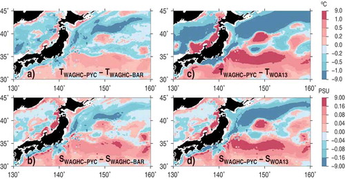
Detailed comparison of the new climatology with the WOA13 atlas highlights the effect of the averaging (interpolation) method. Shown in Figure 1 are the January temperature and salinity difference fields at the 150 m depth level for the high-gradient region of the Kuroshio current east of Japan. The differences between the isopycnally and isobarically averaged WAGHC fields (Figure 1(a,b)) produce spatial patterns similar to the differences between the isopycnally averaged WAGHC and WOA13 (Figure 1(c,d)). Generally, in high-gradient regions the differences may exceed 1°C and 0.2 psu for temperature and salinity respectively for the upper 200 m layer. These differences decrease with depth and essentially vanish below the main thermocline, with the deepest manifestation of this effect (down to about 2000 m) found within the belt of the Antarctic Circumpolar Current.

Figure 1. Differences in (a) temperature and (b) salinity between the isopycnally averaged and isobarically averaged WAGHC climatology in the Kuroshio region at the 150 m level in January. (c, d) As in (a, b) but for the isopycnally averaged WAGHC minus WOA13 differences.

A novel feature of the new climatology is the vertical extrapolation of temperature and salinity profiles. This step is needed because the Argo profiles are limited to the upper 2 km, thus producing a step-like decrease in spatial sampling around this depth. This abrupt change in data coverage creates a strong bias towards the data from the shallower layers when the data are interpolated along isopycnals. The extrapolation method is based on the experimental fact that water properties remain rather stable below the main thermocline and exhibit much weaker lateral gradients compared to the layer above the main thermocline. For the profile reconstruction between the last observed level and the ocean bottom, the adjusted local mean profiles based on the full-depth profiles within a certain geographical vicinity were used. The reconstruction was performed separately for temperature and salinity. The method was applied to about 700,000 Argo and CTD profiles with a maximum observed depth of at least 1500 m.

The automated quality control procedure applied to the original temperature and salinity profiles also differs from the quality control method implemented for the WOA13 atlas. The local climatological parameter ranges are calculated without the assumption of the normal distribution; and the distribution skewness is taken into account according to the method suggested by Vanderviere and Huber (2004). This permits a reduction in the number of potentially good data identified as outliers by the quality control procedure. The selection of the underlying data is also different in these two climatologies. The WOA13 gridded fields represent a blend of six different climatologies compiled for the decadal periods between 1955 and 2012 with 1984 as a median year. For the WAGHC fields, in most cases only the data between 1985 and 2017 were used. For each grid point the median year of the observations is calculated in addition to the main parameters and lies between 2009 and 2011 for the upper 2 km layer and between 2007 and 2009 in the deeper layer. Thus, WAGHC covers a distinctly different and more recent observational period.

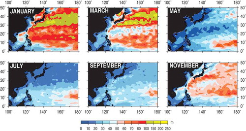
Apart from the temperature and salinity fields at fixed depth levels, WAGHC provides monthly climatological fields of the upper mixed layer depth (MLD) (Gouretski 2018b). These fields were obtained using the optimal interpolation of the MLD determined for each observed profile using the 0.2°C criteria for the temperature difference at two neighboring depth levels. Shown in Figure 2 is a map of the MLD for a part of the western Pacific Ocean for six selected calendar months. Strong interaction between the atmosphere and the ocean in this region is reflected in a profound MLD annual cycle. For instance, East of Japan the mixed layer deepens from 20 to 30 m in summer to more than 200 m in winter.

Figure 2. Upper mixed layer depth in the western Pacific Ocean for six selected calendar months.

4. Conclusions

A new global ocean hydrographic climatology with a considerably larger and more recent database was constructed and is compared here with NOAA’s WOA13 climatology, both with the same temporal and spatial resolution. Differences between the WAGHC and WOA13 climatologies can be attributed mostly to the different spatial interpolation methods and the different data basis. Applying the spatial interpolation procedure to the data on isopycnal surfaces avoids the production of ‘artificial water masses’ and results in a better representation of the temperature salinity relationships in the WAGHC gridded fields. Compared to the WOA13 climatology, the inclusion of the additional data between 2013 and 2018 improved the representation of the thermohaline structure not only for the data-poor polar regions, but also for several areas with apparently sufficient data coverage (the Baltic Sea, Gulf of California, Caribbean Sea, and some other regions). Unsurprisingly, the two climatologies show a high degree of similarity and may be considered as alternative gridded products. WAGHC, however, better describes oceanographic parameters in high-gradient zones and depths. For integral calculations, such as ocean heat content time series, they are nevertheless both useful as a baseline mean.

Acknowledgments

The author gratefully acknowledge helpful discussions with K.P. Koltermann and L. Cheng. The comments from the anonymous reviewer helped to improve the manuscript.

Disclosure statement

No potential conflict of interest was reported by the author.

Additional information

Funding

This work was supported by the Chinese Academy of Sciences President’s International Fellowship Initiative.

References

- Gandin, L. 1963. “Objective Analysis of Meteorological Fields.” Gidrometeorologicheskoe Izdatel’stvo, Leningrad, 242 pp.
- Gouretski, V., and K. Koltermann. 2004. “WOCE Global Hydrograhic Climatology”. Berichte des BSH 35. 52. ISSN: 0946-6010.
- Gouretski, V. 2018a. “World Ocean Circulation Experiment – Argo Global Hydrographic Climatology.” Ocean Science 14: 1127–1146. doi:10.5194/os-14-1127-2018.
- Gouretski, V. 2018b. “WOCE-Argo Global Hydrographic Climatology (WAGHC Version 1.0)”. World Data Center for Climate (WDCC) at DKRZ. doi:10.1594/WDCC/WAGHC_V1.0.
- Koltermann, K. P., V. V. Gouretski, and K. Jancke. 2011. “Hydrographic Atlas of the World Ocean Circulation Experiment (WOCE).” Southampton, UK: International WOCE Project Office.
- Levitus, S. 1982. “Climatological Atlas of the World Ocean.” 173.
- Locarnini, R. A., A. V. Mishonov, J. I. Antonov, T. P. Boyer, H. E. Garcia, O. K. Baranova, M. M. Zweng, and D. R. Johnson. 2010. “World Ocean Atlas 2009, Volume 1: Temperature.” NOAA Atlas NESDIS 68: 184.
- Locarnini, R. A., A. V. Mishonov, J. I. Antonov, T. P. Boyer, H. E. Garcia, O. K. Baranova, M. M. Zweng, et al. 2013. “World Ocean Atlas 2013, In: Volume 1: Temperature.” NOAA Atlas NESDIS 73: 40.
- Lozier, M. S., M. S. McCartnes, and W. B. Owens. 1994. “Anomalous Anomalies in Averaged Hydrographic Data.” Journal of Physical Oceanography 24: 2624–2638. doi:10.1175/1520-0485(1994)024<2624:AAIAHD>2.0.CO;2.
- Roemmich, D., W. J. Gould, and J. Gilson. 2012. “135 Years of Global Ocean Warming between the Challenger Expedition and the Argo Programme.” Nature Climate Change 2: 425–428. doi:10.1038/nclimate1461.
- Roemmich, D., G. C. Johnson, S. Riser, R. Davis, J. Gilson, W. B. Owens, S. L. Garzoli, C. Schmid, and M. Ignaszewski. 2009. “The Argo Program: Observing the Global Ocean with Profiling Floats.” Oceanography 22: 34–43. doi:10.5670/oceanog.2009.36.
- Seidov, D., O. K. Baranova, T. Boyer, S. L. Cross, A. V. Mishonov, and A. R. Parsons. 2016. “Northwest Atlantic Regional Ocean Climatology.” NOAA Atlas NESDIS 80: 56.
- Vanderviere, E., and M. Huber. 2004. “An Adjusted Boxplot for Skewed Distributions.” COMPSTAT’2004 Symposium, Prague, Czech Republic, 1933–1940.