Validation for a tropical belt version of WRF: sensitivity tests on radiation and cumulus convection parameterizations

ABSTRACT

Version 3.9 of WRF-ARW is run with a tropical belt configuration for a period from 2012 to 2016 in this study. The domain covers the entire tropics between 45°S and 45°N with a spatial resolution of about 45 km. In order to verify two radiation schemes and four cumulus convection schemes, eight experiments are performed with different combinations of physics parameterization schemes. The results show that eight experiments present reasonable spatial patterns of surface air temperature and precipitation in boreal summer, with the spatial correlation coefficient (COR) between simulated and observed temperature exceeding 0.95, and that between simulated and observed precipitation ranges from 0.65 to 0.82. The four experiments with the RRTMG radiation scheme show a better performance than the other four experiments with the CAM radiation scheme. In the four experiments with the RRTMG radiation scheme, the COR between simulated and observed surface air temperature is about 0.98, and that between simulated and observed precipitation ranges from 0.76 to 0.82. Comparatively, the two experiments using the new Tiedtke cumulus parameterization scheme can simulate better diurnal variation of precipitation in boreal summer than the other six experiments. In particular, for the diurnal cycle of precipitation over land and ocean, the experiment using the RRTMG radiation scheme and the new Tiedtke cumulus convection scheme shows that the peaks of precipitation rate appear at 0400 LST and 1600 LST, in agreement with observation.

Graphical Abstract

摘要

对基本气候态和降水日变化的分析是检验模式模拟性能、理解模式误差来源的重要手段。为了评估出对热带气候模拟效果较好的物理参数化方案组合，本文应用WRF带状区域模式，主要比较了四种积云对流参数化方案: New Tiedtke、Kain-Fritsch、new SAS、Tiedtke，和两种辐射参数化方案: RRTMG和CAM，对热带带状区域的气候模拟结果。研究表明：使用New Tiedtke积云对流参数化方案和RRTMG辐射方案的试验，表现出对气温、降水及降水日变化等综合性最好的模拟性能；New Tiedtke积云对流参数化方案能模拟出较好的降水空间分布和降水日变化位相分布特征；与RRTMG辐射方案相比，CAM辐射方案会使温度模拟偏低，特别是陆地上更明显，这种陆地上的冷偏差可能主要来源于T_min的模拟偏冷。

KEYWORDS:

• WRF model
• cumulus convection parameterization
• radiation scheme
• diurnal cycle of precipitation

关键词:

• WRF 模式，积云对流参数化方案，辐射参数化方案，降水日变化

1. Introduction

Regional Climate Models (RCMs) have been widely applied to present-day climate simulation and climate change projection, and most of these applications are run with a limited area domain setting (Giorgi and Shields 1999; Giorgi et al. 2012). As a special domain setting, a tropical belt configuration has been used in a few studies to explore a range of processes related to tropical climate interactions and assess the performance of given physics parameterization schemes in a wide range of climate contexts (Tulich, Kiladis, and Suzuki-Parker 2011; Ray et al. 2011; Coppola et al. 2012). These regional climate studies for a tropical belt used either the WRF model or RegCM. The main results can be summarized as follows: Both models can basically simulate the features of surface climate, i.e. the relatively narrow strip of rain across the central North Pacific and local rainfall enhancements near the Western Ghats of India, as well as capture the precipitation anomaly patterns for ENSO or the MJO. However, there are quite large biases over most regions, e.g. the ITCZ over the eastern Pacific is displaced a few degrees north and a significant wet bias is situated over the Indian subcontinent during summer. These biases may be due to joint effects – specifically, a combination of several model physics parameterization schemes and a lack of model tuning (Murthi, Bowman, and Leung 2011).

The performance in simulating tropical precipitation is highly sensitive to the physics parameterization schemes, especially cumulus convection schemes and radiation parameterization schemes (Fowler and Randall 2002). Clouds, convection, and their radiative properties play important roles in determining global climate. In particular, these related processes result in nonlinear effects on atmospheric circulation. Different cumulus convection parameterization schemes have different impacts not only on the hydrological cycle through precipitation and evaporation, but also on the large-scale flow by the release of latent heat and vertical transport of sensible heat, water vapor, and momentum (Yao and Genio 1999; Arakawa 2004; Yang et al. 2015).

To date, very few studies have used the WRF model with a tropical belt configuration. For a tropical belt simulation, an RCM is less strongly influenced by lateral boundary condition forcing than in its typical limited area domain configuration (Coppola et al. 2012). In order to simulate the tropical climate well by using WRF, the key issue is to choose appropriate physics parameterization schemes. Here, we use the WRF modeling system to conduct eight sensitivity experiments, by combining four cumulus parameterization schemes and two radiation schemes. Specifically, we focus on validating the spatial distribution of surface air temperature at a height of 2 m (hereinafter referred to as T_2m) and precipitation, as well as the diurnal cycle of precipitation. Since there is a stronger diurnal cycle of precipitation over much of the globe in boreal summer compared to the other three seasons (Dai 2001), we choose boreal summer as the studied season.

The remainder of the paper is structured as follows: In Section 2 we provide a brief presentation of the WRF model and the forcing and observation data used in this study. In Section 3 we analyze the results of the simulations. A summary and discussion are given in Section 4.

2. Model and data

2.1. Model setting

WRF-ARW is developed by the Mesoscale and Microscale Meteorology Division of the National Center for Atmospheric Research and is widely used for weather forecasting and regional climate modeling studies (Skamarock et al. 2008).

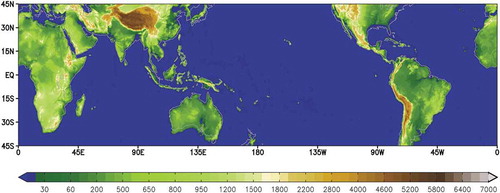
In this work, we use version 3.9 of WRF-ARW with a tropical belt configuration in which the periodic boundary condition is configured in the east–west direction. The model is integrated continuously for five years, from 1 January 2012 to 31 December 2016. The integration runs on Mercator projection grids, and the model outputs at an hourly interval. The domain, shown in Figure 1, spans the entire tropical belt between 45°S and 45°N, with a spatial resolution of 45 km. The choice of using a resolution of 45 km is aimed at obtaining an appropriate combination of physical parameterizations for later use in our global climate model, which is going to take part in the HighResMIP project (Haarsma et al. 2016). There are 51 vertical levels, and the model top is at 10 hPa.

Figure 1. The domain used in this study and the topography (units: m).

Table 1 shows the configurations of different physics parameterization schemes in all the eight WRF experiments. The schemes include cumulus convection, radiation, microphysics, surface layer, land surface, and PBL, and have been used popularly in previous WRF studies (Murthi, Bowman, and Leung 2011; Gbode et al. 2018).

Table 1. Configurations of physics parameterization schemes used in our eight experiments.

Parameterization scheme	Experiment
	a1	b1	c1	d1	a2	b2	c2	d2
Cumulus convection	New Tiedtke	KF	New SAS	Tiedtke	New Tiedtke	KF	New SAS	Tiedtke
Radiation	RRTMG				CAM
Microphysics	WSM6 (Hong and Lim 2006)
Surface layer	MM5 (Beljaars 2010)
Land surface	Noah (Tewari et al. 2004)
PBL	YSU (Hong, Noh, and Dudhia 2006)

Notes: KF, Kain–Fritsch; New SAS, new Simplified Arakawa–Schubert scheme from Yonsei University; RRTMG, Rapid Radiative Transfer Model for global models; CAM, Community Atmosphere Model; WSM6, WRF Single-Moment 6-class scheme; MM5, Revised MM5 surface layer scheme; Noah, Unified Noah land-surface model; YSU, Yonsei University Planetary Boundary Layer Parameterization.

In this study, we focus on verifying two radiation and four cumulus convection schemes. The two radiation schemes used are CAM (Collins et al. 2004) and RRTMG (Iacono et al. 2008). The CAM scheme uses a Delta-Eddington approximation for shortwave radiation absorption and scattering, and the RRTMG scheme uses the correlated-k method for radiative transfer. The four cumulus convection parameterizations used are Tiedtke (Tiedke 1989; Zhang, Wang, and Hamilton 2011), new Tiedtke (Zhang and Wang. 2017), KF (Kain 2004), and New SAS (Han and Pan 2011). The Tiedtke scheme is a mass-flux scheme with a CAPE closure. It considers three types of convection: penetrative, shallow, and midlevel. The new Tiedtke scheme has modified trigger functions for deep and shallow convection, and allows the CAPE to relax to a value from the PBL (Bechtold et al. 2014; Owens and Hewson 2018). The KF scheme is also a mass-flux scheme with CAPE closure, but it has different triggers and the details of the closure is different (Kain 2004). The new SAS scheme produces more intense deep convection, and its shallow component now employs a mass-flux approach, instead of a diffusion method (Han and Pan 2011). Since the WRF model adds and updates new and existing physical parameterizations every half-year, our experiments are mainly designed to test new physics options in WRF-ARW version 3.9.

2.2. Data

The forcing conditions used for the northern and southern boundaries in all eight experiments are from ERA-Interim (Dee et al. 2011), and these are the SST fields. The bottom and lateral boundary conditions are updated at six-hour intervals at a spatial resolution of 1.5° × 1.5°.

The observational dataset employed to validate the simulated surface air temperature is from ERA-Interim data with a spatial resolution of 1.5° × 1.5° and CRU data with a spatial resolution of 0.5° × 0.5°, which is available for land points. The observational precipitation data are obtained from CMORPH satellite rainfall products (Joyce et al. 2004). Previous research has demonstrated the reliability of CMORPH data (Janowiak, Kousky, and Joyce 2005; Yang and Yi 2014; Kumar, Patra, and Lakshmi 2016). Compared with TRMM or GPCP data, the CMORPH dataset has a higher spatial and temporal resolution. The available coverage of CMORPH data extends from 60°S to 60°N, with a spatial resolution of 0.07275° × 0.07277° and a temporal resolution of 0.5 h. CMORPH data are used to validate both the spatial distribution and the diurnal cycle of the simulated precipitation, after horizontal interpolation to the model grid.

In analyzing the diurnal cycle for precipitation, the calculated climatological precipitation rate for UTC is converted to the corresponding local solar time (LST), based on the longitude where the grid points are located. The phase of the diurnal cycle refers to the time when the peaks of precipitation rate appear; the amplitude of the diurnal cycle means the value of maximum precipitation rate (Dai 2001; Zhang, Bi, and Kong 2015).

3. Results

3.1. Spatial distribution of surface air temperature

Figure 2 shows the spatial distributions of mean T_2m from observation and the mean T_2m biases between simulation and observation in boreal summer. The spatial distribution of observed mean T_2m from ERA-Interim is shown in Figure 2(a), and that from CRU are in Figure 2(f). The spatial correlation of T_2m between ERA-Interim and CRU is 0.997. The spatial distributions of observed mean T_2m reveal that the surface air temperature decreases latitudinally from the equator to high latitudes. Several warm centers are mainly located in the desert regions of the Sahel, Arabia, South Asia etc., and two cold centers are clearly located over the Tibetan Plateau and Andes mountain range. For all eight experiments, the spatial correlation coefficient (COR) of T_2m between simulation and observation exceeds 0.95, which indicates that the spatial pattern of T_2m is simulated quite well.

Figure 2. Spatial distributions of mean observed surface air temperature (units: °c) from (a) ERA-Interim and (f) CRU, and the (b–e, g–j) mean biases of surface air temperature (units: °c) between simulation and observation (ERA-Interim) in boreal summer. Values in the upper-left corners are the spatial correlation coefficient with ERA-Interim; values in the upper-right corner are the mean bias and RMSE between simulation and observation (ERA-Interim).

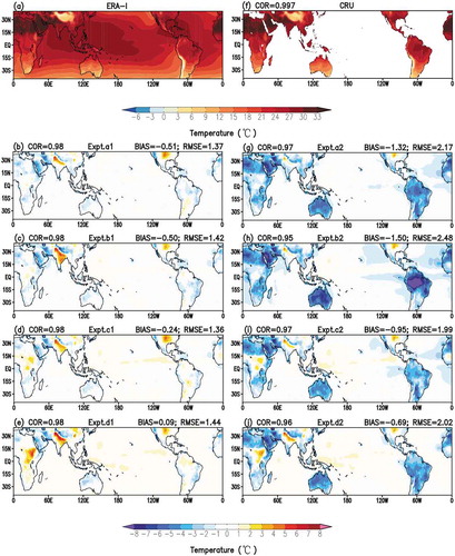
However, for the four experiments with the CAM radiation scheme (a2, b2, c2 and d2), the COR between simulation and observation is lower than that for the other experiments, and the pattern of mean T_2m bias displays a clear cold bias over most land regions. It is found that both daily maximum and daily minimum T_2m present certain cold biases, but the daily mean T_2m cold biases are mainly due to the daily minimum 2 m air temperature over land (figure not shown). This agrees with the previous research of Abdallah et al. (2015).

Among the four experiments with the RRTMG radiation scheme (a1, b1, c1 and d1), the RMSEs between simulation and observation in a1 and c1 are approximately equal to 1.36, and are less than those in b1 and d1, which indicates that the T_2m could be better simulated in the experiments using either the new Tiedtke or the new SAS cumulus convection parameterization scheme.

3.2. Spatial distribution of precipitation

Figure 3 shows the spatial distribution of precipitation from observation and simulation in boreal summer. The observed basic spatial patterns for tropical precipitation are shown in Figure 3(a), such as the heavy rainfall belts around the Philippines and Indonesia, and a narrow belt of maximum precipitation to the north of the equator (i.e. the ITCZ). Figure 3(b–i) show that the precipitation distribution patterns are generally simulated well. For the eight experiments, the COR of precipitation between simulation and observation is 0.80, 0.76, 0.82, 0.78, 0.70, 0.65, 0.75, and 0.66, respectively. However, the total precipitation is overestimated in all eight experiments. Meanwhile, the mean precipitation biases between observation and simulation (not shown) depict deficiencies in simulated regional features in all runs. The deficiencies include an incorrect ITCZ rain-belt breadth across the entire tropical Pacific, overestimated precipitation over eastern Indo-Pacific regions, and underestimated precipitation over most of the eastern Pacific Ocean. These biases have also been found in previous WRF research (Katragkou et al. 2015; Gbode et al. 2018).

Figure 3. Spatial distribution of mean precipitation (units: mm d⁻¹) from (a) observation (CMORPH) and (b–i) simulation in boreal summer. Values in the upper-left corner are the spatial correlation coefficients between simulation and observation; values in the upper-right corner are the mean precipitation and RMSE between simulation and observation.

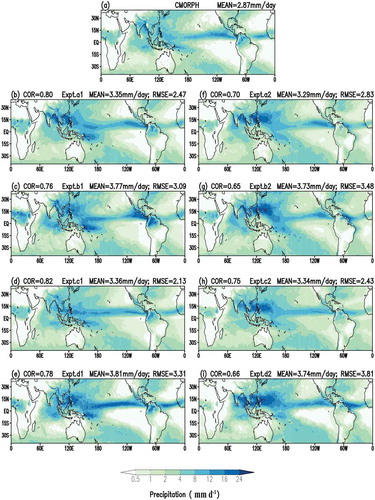
The COR for precipitation between simulation and observation is larger in the four experiments with the RRTMG radiation scheme (a1, b1, c1 and d1) than those in the four experiments with the CAM scheme (a2, b2, c2, and d2). Among the four experiments using the RRTMG radiation scheme, the experiments using the new Tiedtke (a1) and the new SAS (c1) cumulus convection schemes present a higher COR between simulation and observation than the other two experiments. For these two experiments, the simulated mean values of precipitation are also closer to the observed.

3.3. Diurnal cycle of precipitation

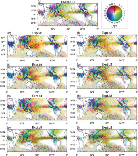
Figure 4 presents the mean diurnal cycle of precipitation from observation (CMORPH data) and from simulation in boreal summer. The color shading indicates the LST when the maximum precipitation rate appears (precipitation phase), ranging from 0000 LST to 2300 LST. The intensity of the color saturation represents the magnitude of the maximum precipitation rate (precipitation amplitude). Mean precipitation rates of less than 0.12 mm d⁻¹ are neglected in calculating the diurnal cycle of precipitation.

Figure 4. Spatial distribution of the diurnal cycle of precipitation from (a) observation (CMORPH) and (b–i) simulation in boreal summer. The color shading indicates the LST when the maximum precipitation appears, while The intensity of color indicates the magnitude of the maximum precipitation rate (units: mm d⁻¹). Mean precipitation rates less than 0.12 mm d⁻¹ are neglected.

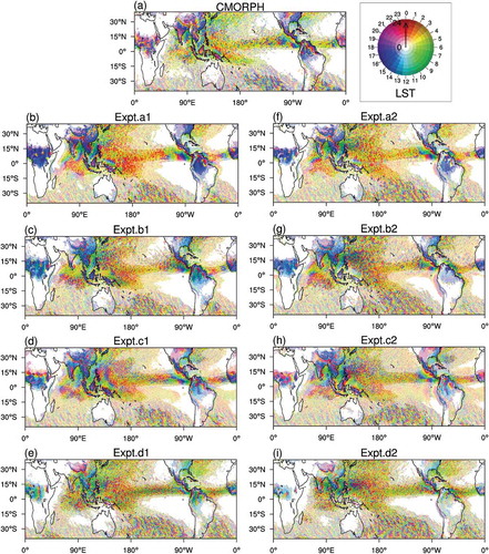
The observed features for the diurnal cycle of precipitation in boreal summer are shown in Figure 4(a). The maximum precipitation rate over inland regions tends to occur during afternoon or night (1300–2200 LST); additionally, the maximum precipitation rate over ocean and small island areas happens usually during night or early morning (0000–0700 LST), and these features are mainly caused by the land–sea contrast (Dai 2001, 2006). As shown in Figure 4(b–i), the amplitude of the diurnal maximum precipitation rate is simulated well in all eight experiments, except that the simulated maximum precipitation rate occurs prematurely over most land regions. In particular, in the two experiments with the Tiedtke cumulus convection scheme (d1 and d2), the simulated maximum precipitation rate occurs 5 h ahead of observation. Comparatively, the precipitation phases simulated in the two experiments using the new Tiedtke cumulus convection scheme (a1 and a2) are in better agreement with observation. One possible reason is that the new Tiedtke cumulus convection scheme can realistically represent tropical convectively coupled waves and synoptic variability with use of the extended CAPE closure (Bechtold et al. 2014).

In order to carry out further comparative analysis with respect to the features of land–sea contrast, the diurnal cycle of precipitation is presented using a diurnal anomaly plot. Figure 5 shows the composite diurnal cycle of precipitation averaged from observation and simulation in boreal summer between 25°S and 25°N, over the whole tropical domain, land and ocean, respectively. Figure 5(a) presents large differences in the diurnal cycle of precipitation between observation and simulation over the whole domain. There are two precipitation-rate peaks observed, shown as a semidiurnal wave pattern superimposed on a diurnal wave. One early-morning precipitation rate peak occurs at 0400 LST, and the other afternoon precipitation rate peak occurs at 1600 LST. Among all eight experiments, the case run with the RRTMG radiation scheme and the new Tiedtke cumulus convection scheme (a1) most successfully simulates this kind of precipitation phase. However, almost all experiments overestimate the afternoon precipitation rate peak—even the experiment with the new Tiedtke scheme.

Figure 5. Composite diurnal cycle of precipitation between 25°S and 25°N in boreal summer (units: %) over (a) the whole tropical domain, (b) land, and (c) ocean. The vertical coordinate represents the percentage of the maximum precipitation rate deviation from its average. Black solid line: observed precipitation; colored solid lines: four experiments with the RRTMG radiation scheme; colored dashed lines: four experiments with the CAM radiation scheme.

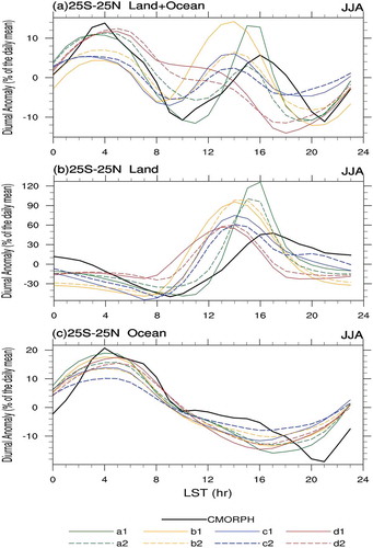
As shown in Figure 5(b,c), the observed precipitation peak occurs in the afternoon over land and in the early morning over ocean, respectively. These features are consistent with previous studies (Dai 2001, 2006; Zhang, Bi, and Kong 2015; Li, Bi, and Zhang 2018). Among all eight experiments, comparatively, the experiment using the RRTMG radiation scheme and the new Tiedtke cumulus convection scheme performs best, albeit with some differences in the amplitude and phase of the simulated maximum precipitation rate. The simulated maximum precipitation rate over land occurs from 1300 to 1600 LST, and the time is about 1–4 h ahead of observation, except in the two experiments with the new Tiedtke cumulus convection scheme. The time when the maximum precipitation rate occurs is simulated much better over ocean than over land, and all the simulated maximum precipitation rates over the ocean occur within 0500–0600 LST.

4. Summary

Validation of the basic climatology and the diurnal cycle of precipitation is an important task for model development. In order to verify the impacts of radiation and cumulus convection physics parameterization schemes, we carry out eight WRF experiments, with a tropical belt configuration, and each experiment is run with a different physics parameterization scheme configuration. Our study focuses mainly on analyzing the spatial patterns of surface air temperature, precipitation, and the diurnal cycle of precipitation in boreal summer.

The simulated surface air temperature in boreal summer is obviously sensitive to the radiation scheme. The spatial distribution of surface air temperature is successfully simulated in all the experiments, with the COR between simulation and observation ranging from 0.95 to 0.98. Also, the four experiments with the RRTMG radiation scheme show a higher COR with observation and smaller RMSE between simulation and observation, than those experiments with the CAM radiation scheme.

The basic spatial pattern of tropical precipitation in boreal summer is reproduced well in all simulations, such as the narrow belt of maximum precipitation rate to the north of the equator. Among all eight experiments, the spatial distribution of precipitation could be better simulated in the experiments using either the new Tiedtke or the new SAS cumulus convection parameterization scheme, but the experiment with the new SAS scheme cannot represent the diurnal cycle of precipitation well.

With regards to the diurnal cycle of precipitation, the observed maximum precipitation rate occurs more frequently in the afternoon over land, and in the early morning over ocean. Among all eight experiments, the experiment with the RRTMG radiation scheme and the new Tiedtke cumulus convection scheme performs best, with a COR between simulation and observation of 0.80, and the simulated maximum precipitation rate occurring at 0400 LST and 1600 LST. Though the experiment with the new Tiedtke scheme produces a better diurnal cycle, it overestimates the strength of the maximum precipitation rate.

In future work we will further verify the impact of physics parameterization schemes in simulating the tropical and extratropical rainbelt, and attempt to implement the most suitable physical parameterization option identified into our global model for the HighResMIP project.

Disclosure statement

No potential conflict of interest was reported by the authors.

Additional information

Funding

This work was supported by the National Key Research Program of China [grant number 2016YFB0200805) and the National Natural Science Foundation of China [grant number 41575089].

References

- Abdallah, A., M. M. Eid, M. M. Wahab, and F. M. Elhussainy. 2015. “Regional Climate Simulation of WRF Model over North Africa: Temperature and Precipitation.” World Environment 5 (4): 160–173. doi:10.5923/j.env.20150504.04.
- Arakawa, A. 2004. “The Cumulus Parameterization Problem: Past, Present, and Future.” Journal of Climate 17 (13): 2493–2525. doi:10.1175/1520-0442(2004)017<2493:ratcpp>2.0.co;2.
- Bechtold, P., N. Semane, P. Lopez, J. P. Chaboureau, A. Beljaars, and N. Bormann. 2014. “Representing Equilibrium and Nonequilibrium Convection in Large-Scale Models.” Journal of Atmospheric Sciences 71 (2): 734–753. doi:10.1175/JAS-D-13-0163.1.
- Beljaars, A. C. M. 2010. “The Parametrization of Surface Fluxes in Large‐Scale Models under Free Convection.” Quarterly Journal of the Royal Meteorological Society 121 (522): 255–270. doi:10.1002/qj.49712152203.
- Collins, W., Rasch, P. J., Boville, B. A., McCaa, J., Williamson, D. L., Kiehl, J. T., and Briegleb, B. P., et al., 2004: “Description of the NCAR Community Atmosphere Model (CAM 3.0)”. NCAR Technical Note, NCAR/TN–464+STR. doi:10.5065/D63N21CH.
- Coppola, E., F. Giorgi, L. Mariotti, and X. Bi. 2012. “RegT-Band: A Tropical Band Version of RegCM4.” Climate Research 52 (1): 115–133. doi:10.3354/cr01078.
- Dai, A. 2001. “Global Precipitation and Thunderstorm Frequencies. Part II: Diurnal Variations.” Journal of Climate 14 (6): 1092–1111. doi:10.1175/1520–0442(2001)014<1112:gpatfp>2.0.co;2.
- Dai, A. 2006. “Precipitation Characteristics in Eighteen Coupled Climate Models.” Journal of Climate 19 (18): 4605–4630. doi:10.1175/JCLI3884.1.
- Dee, D. P., S. Uppala, A. Simmons, P. Berrisford, P. Poli, S. Kobayashi, U. Andrae, et al. 2011. “The ERA-Interim Reanalysis: Configuration and Performance of the Data Assimilation System.” Quarterly Journal of the Royal Meteorological Society 137 :553–597. doi:10.1002/qj.828.
- Fowler, L. D., and D. A. Randall. 2002. “Interactions between Cloud Microphysics and Cumulus Convection in a General Circulation Model.” Journal of Atmospheric Sciences 59 (21): 3074–3098. doi:10.1175/1520-0469(2002)059<3074:IBCMAC>2.0.CO;2.
- Gbode, I. E., J. Dudhia, K. O. Ogunjobi, and V. O. Ajayi. 2018. “Sensitivity of Different Physics Schemes in the WRF Model during a West African Monsoon Regime.” Theoretical and Applied Climatology. doi:10.1007/s00704-018–2538–x.
- Giorgi, F., E. Coppola, F. Solmon, L. Mariotti, M. B. Sylla, X. Bi, N. Elguindi, et al. 2012. “RegCM4: Model Description and Preliminary Tests over Multiple CORDEX Domains.” Climate Research 52 :7–29. doi:10.3354/cr01018.
- Giorgi, F., and C. Shields. 1999. “Tests of Precipitation Parameterizations Available in Latest Version of NCAR Regional Climate Model (Regcm) over Continental United States.” Journal of Geophysical Research Atmospheres 104 (D6): 6353–6375. doi:10.1029/98JD01164.
- Haarsma, R. J., M. J. Roberts, P. L. Vidale, C. A. Senior, A. Bellucci, Q. Bao, P. Chang, et al. 2016. “High Resolution Model Intercomparison Project (Highresmip V1.0) For CMIP6.” Geoscientific Model Development Discussions 9 (11): 4185–4208. doi:10.5194/gmd-9–4185-2016.
- Han, J., and H. L. Pan. 2011. “Revision of Convection and Vertical Diffusion Schemes in the NCEP Global Forecast System.” Weather and Forecasting 26 (4): 520–533. doi:10.1175/waf-d-10-05038.1.
- Hong, S. Y., and J. O. J. Lim. 2006. “The WRF Single-Moment 6-Class Microphysics Scheme (WSM6).” Journal of Korean Meteorological Society 42 (2): 129–151.
- Hong, S. Y., Y. Noh, and J. Dudhia. 2006. “A New Vertical Diffusion Package with an Explicit Treatment of Entrainment Processes.” Monthly Weather Review 134 (9): 2318. doi:10.1175/MWR3199.1.
- Iacono, M. J., J. S. Delamere, E. J. Mlawer, M. W. Shephard, S. A. Clough, and W. D. Collins. 2008. “Radiative Forcing by Long‐Lived Greenhouse Gases: Calculations with the AER Radiative Transfer Models.” Journal of Geophysical Research Atmospheres 113: D13. doi:10.1029/2008JD009944.
- Janowiak, J. E., V. E. Kousky, and R. J. Joyce. 2005. “Diurnal Cycle of Precipitation Determined from the CMORPH High Spatial and Temporal Resolution Global Precipitation Analyses.” Journal of Geophysical Research Atmospheres 110 (D23). doi:10.1029/2005JD006156.
- Joyce, R. J., J. E. Janowiak, P. A. Arkin, and P. Xie. 2004. “CMORPH: A Method that Produces Global Precipitation Estimates from Passive Microwave and Infrared Data at High Spatial and Temporal Resolution.” Journal of Hydrometeorology 5 (3): 487–503. doi:10.1175/1525-7541(2004)005<0487:camtpg>2.0.co;2.
- Kain, J. S. 2004. “The Kain Fritsch Convective Parameterization: An Update.” Journal of Applied Meteorology 43 (1): 170–181. doi:10.1175/1520-0450(2004)043<0170:tkcpau>2.0.co;2.
- Katragkou, E., M. Garcíadíez, R. Vautard, S. Sobolowski, P. Zanis, G. Alexandri, R. M. Cardoso, et al. 2015. “Regional Climate Hindcast Simulations within EURO-CORDEX: Evaluation of a WRF Multi-Physics Ensemble.” Geoscientific Model Development 8 (3): 603–618. doi:10.5194/gmd-8-603-2015.
- Kumar, B., K. C. Patra, and V. Lakshmi. 2016. “Daily Rainfall Statistics of TRMM and CMORPH: A Case for Trans-Boundary Gandak River Basin.” Journal of Earth System Science 125 (5): 919–934. doi:10.1007/s12040-016-0710-1.
- Li, X. Y., X. Q. Bi, and H. Zhang. 2018. “Evaluation of NCAR CESM and CAS ESM Models for the Simulation of Boreal Summer Climate over Eastern Asia: Climatological Mean and Diurnal Cycle of Precipitation.” Climatic and Environmental Research(In Chinese) 23 (6): 645–656. doi:10.3878/j.issn.1006-9585.2018.18050.
- Murthi, A., K. P. Bowman, and L. R. Leung. 2011. “Simulations of Precipitation Using NRCM and Comparisons with Satellite Observations and CAM: Annual Cycle.” Climate Dynamics 36 (9): 1659–1679. doi:10.1007/s00382-010-0878-z.
- Owens, R. G., and T. D. Hewson. 2018. “ECMWF Forecast User Guide.” Reading: ECMWF. doi:10.21957/m1cs7h.
- Ray, P., C. Zhang, M. W. Moncrieff, J. Dudhia, J. M. Caron, and C. Bruyere. 2011. “Role of the Atmospheric Mean State on the Initiation of the Madden-Julian Oscillation in a Tropical Channel Model.” Climate Dynamics 36 (1): 161–184. doi:10.1007/s00382-010-0859-2.
- Skamarock, W. C., J. B. Klemp, J. Dudhia, D. O. Gill, D. M. Barker, M. G. Duda, X. Y. Huang, et al., 2008: “A Description of the Advanced Research WRF Version 3”. NCAR Technical Note NCAR/TN-475+STR. doi:10.5065/D68S4MVH.
- Tewari, M., F. Chen, W. Wang, J. Dudhia, M. A. Lemone, K. Mitchell, M. Ek, et al., 2004: “Implementation and Verification of the Unified NOAH Land Surface Model in the WRF Model.” 20th Conference on Weather Analysis and Forecasting/16th Conference on Numerical Weather Prediction, American Meteorological Society, Seattle, WA, US.
- Tiedke, M. A. 1989. “A Comprehensive Mass Flux Scheme for Cumulus Parameterization in Largescale Models.” Monthly Weather Review 117 (8): 1779–1800. doi:10.1175/1520-0493(1989)117<1779:acmfsf>2.0.co;2.
- Tulich, S. N., G. N. Kiladis, and A. Suzuki-Parker. 2011. “Convectively Coupled Kelvin and Easterly Waves in a Regional Climate Simulation of the Tropics.” Climate Dynamics 36 (1): 185–203. doi:10.1007/s00382-009-0697-2.
- Yang, B., Y. Zhang, Y. Qian, T. Wu, A. Huang, and Y. Fang. 2015. “Parametric Sensitivity Analysis for the Asian Summer Monsoon Precipitation Simulation in the Beijing Climate Center AGCM Version 2.1.” Journal of Climate 28 (14): 5622–5644. doi:10.1175/JCLI-D-14-00655.1.
- Yang, Y., and L. Yi. 2014. “Evaluating the Performance of Remote Sensing Precipitation Products CMORPH, PERSIANN, and TMPA, in the Arid Region of Northwest China.” Theoretical and Applied Climatology 118 (3): 429–445. doi:10.1007/s00704-013-1072-0.
- Yao, M. S., and D. A. D. Genio. 1999. “Effects of Cloud Parameterization on the Simulation of Climate Changes in the GISS GCM.” Journal of Climate 12 (3): 761–779. doi:10.1175/1520-0442(1999)012<0761:EOCPOT>2.0.CO;2.
- Zhang, C., Y. Wang, and K. Hamilton. 2011. “Improved Representation of Boundary Layer Clouds over the Southeast Pacific in ARW-WRF Using a Modified Tiedtke Cumulus Parameterization Scheme.” Monthly Weather Review 139 (11): 3489–3513. doi:10.1175/MWR-D-10-05091.1.
- Zhang, C., and Y. Wang. 2017. “Projected Future Changes of Tropical Cyclone Activity over the Western North and South Pacific in a 20-Km-Mesh Regional Climate Model.” Journal of Climate 30 (15): 5923–5941. doi:10.1175/JCLI-D-16-0597.1.
- Zhang, X. X., X. Q. Bi, and X. H. Kong. 2015. “Observed Diurnal Cycle of Summer Precipitation over South Asia and East Asia Based on CMORPH and TRMM Satellite Data.” Atmospheric and Oceanic Science Letters 8 (4): 201–207. doi:10.3878/AOSL20150010.