In-situ measurement of CO₂ at the Xinglong regional background station over North China

ABSTRACT

High-accuracy continuous measurements of atmospheric concentrations of CO₂ were made from May 2016 to December 2017 using the Picarro G2301 analyzer at Xinglong station (40°24′N, 117°30′E, 940 MSL), 150 km northeast of Beijing. The near-ground CO₂ measurements were calibrated by standards based on WMO procedures. The regional background measurements were filtered by the robust extraction of baseline signal method to study the seasonal and diurnal cycles. The regional background CO₂ concentrations were low in summer. The maximum difference between the local sources and regional background CO₂ concentrations occurred in summer and autumn, indicating a strong influence from local sources. Cluster analysis and potential source contribution function analysis showed that the long-distance transport of anthropogenic emissions in the Beijing–Tianjin–Hebei metropolitan area influenced the CO₂ concentrations in Xinglong, especially in summer. The diurnal variation of CO₂ was mainly influenced by the various vertical transport conditions of the tropospheric atmosphere in a day.

Graphical abstract

摘要

基于兴隆站Picarro G2301观测资料，本文分析了2016年5月至2017年12月近地面二氧化碳浓度变化趋势以及远距离输送的影响。采用背景值筛选方法，提取了兴隆站二氧化碳背景浓度和污染浓度。分析表明，兴隆站二氧化碳背景浓度和污染浓度有相似的季节变化特征，夏季最低，冬季和早春较高。冬季和早春的高背景值主要由于正的生物通量，即更强的植物呼吸作用和更弱的植物光合作用；夏季则相反，夏季和初秋污染浓度与背景浓度差值均较大，主要是本地源排放增加，而72小时后向轨迹的聚类分析以及PSCF分析也表明，夏季由于来自北京，天津，河北和山东的气流输送，携带有高浓度二氧化碳气团也会使兴隆地区的二氧化碳污染浓度升高。远距离输送结果也表明，京津冀区域人为排放二氧化碳对兴隆地区四个季节的二氧化碳浓度均有正的贡献，冬季来自内蒙古和张家口的气团输送也会带来正的贡献。二氧化碳浓度的日变化在所有季节都很显著， 10:00至14:00左右二氧化碳浓度较低。中午较强的边界层对流将高空低浓度的二氧化碳向下输送到近地面大气，下午则相反，而高值通常发生在夜间。

KEYWORDS:

• Xinglong station
• CO₂ concentration
• variation
• source analysis

关键词:

• 兴隆站
• CO₂浓度
• 变化趋势
• 远距离输送

1. Introduction

The continuous increases in the concentrations of greenhouse gases, particularly CO₂, have attracted much attention from the international community. The global average concentration of atmospheric CO₂ has increased by 145% since the pre-industrial era and was up to 403.3 ± 0.1 ppm in 2016 (WMO 2017). CO₂ has a long lifetime in the atmosphere and contributes >60% of the total radiative forcing of greenhouse gases, although it accounts for a relatively small proportion of the total amount of gas in the atmosphere (IPCC 2013). The increase in atmospheric concentrations of CO₂ is mainly attributed to the burning of fossil fuels and changes in land use (Peters et al. 2011). The sources and sinks of CO₂ in the atmosphere are unevenly distributed and subject to a variety of transport processes. High-precision measurements of the concentrations of CO₂ provide a foundation for the assessment of carbon emissions and studies of the carbon cycle (Andrews et al. 2014; Fang et al. 2014).

Governments and research groups have put much effort into monitoring and quantifying the magnitude and distribution of greenhouse gases at both domestic and international levels. To date, there are more than 150 sites worldwide in the World Meteorology Organization/Global Atmosphere Watch (WMO/GAW) network, with the aim of detecting changes in greenhouse gas concentrations and source–sink analysis. The USA has conducted long-term observations of atmospheric CO₂ concentrations at the Mauna Loa site in Hawaii since 1958. The US National Oceanic and Atmospheric Administration (NOAA) Earth System Research Laboratory have been working to build a network of tall-tower CO₂ measurement sites since the early 1990s (Bakwin et al. 1998; Zhao, Bakwin, and Tans 1997) and a reliable and precise in-situ CO₂ analysis system has been developed and deployed at eight sites in the NOAA Earth System Research Laboratory Global Greenhouse Gas Reference Network. The Integrated Carbon Observation System in Europe is committed to providing high-precision data to determine the spatial distributions of long-term changes in CO₂ concentrations (Yver Kwok et al. 2015).

The concentrations of greenhouse gases in China are increasing quickly due to rapid economic growth and the increased combustion of fossil fuels. Since the 1990s, seven CO₂/CH₄ background stations have been set up by the China Meteorological Administration (CMA), and four of them — Waliguan in Qinghai Province, Shangdianzi in Beijing, Lin’an in Zhejiang Province, and Longfeng Mountain in Heilongjiang Province (Fang et al. 2014; Liu et al. 2009) — belong to the WMO/GAW global network.

Measurements of CO₂ in economically developed and densely populated areas of China are important due to the impact of human activities, especially in the Beijing–Tianjin–Hebei metropolitan area. Xinglong station is located in Xinglong County, Hebei Province, and can be used as a background station for the Beijing–Tianjin–Hebei metropolitan area (Cheng et al. 2003). A Picarro cavity ring-down spectroscopy (CRDS) analyzer is used for monitoring carbon emissions.

2. Data and methods

2.1. In-situ measurement methods

Xinglong station (40°24′N, 117°30′E, 940 MSL) (red spot in Figure S1) is located in Xinglong County, Hebei Province, south of the Yanshan Mountains, about 150 km northeast of Beijing. It is surrounded by mountains with shrubland and grassland. Also, there are no industrial activities within 20 km. Xinglong station is far from megacities and major transport routes and the atmospheric conditions may, therefore, represent the regional atmosphere (Wu et al. 2010).

Based on CRDS techniques, the Picarro instrument is designed as a low drift, high-precision greenhouse gas analyzer. The intensity of the laser introduced into a high-precision optical cavity decays exponentially with time. The decay time constant, τ, depends on the loss during the transport between different endoscopes in the optical cavity and the absorption and scattering of the sample being measured. The concentration of the gas sample is related to τ (Crosson 2008). CO₂ concentrations have been observed at Xinglong station using the Picarro G2301 high-precision CRDS analyzer since May 2016. The instrument sampling inlet is located on the roof of a three-story building and has been operated for more than 1 year.

2.2. Data processing

2.2.1. Calibration

Eight calibrations were performed from 14 November to 14 December 2017, with a duration of 15 min for each calibration, to determine the stability of the G2301 high-precision CRDS analyzer. Standard gas, with a CH₄ concentration of 2036.5 ± 0.3 ppb and a CO₂ concentration of 399.95 ± 0.02 ppm under dry and clean atmospheric conditions was calibrated by the Meteorological Observation Center of the CMA based on the WMO X2007 scale for CO₂.

The response of the analyzer is unstable after the start of calibration as a result of the time required for flushing the internal volume of the analyzer (Yan et al. 2011). We set the flushing time to 5 min and therefore only data obtained 5 min after the start of the calibration were retained. The temporal resolution of the raw data was 5 s, but 1-min average values were used for the calibration analysis and 1-h average values elsewhere.

2.2.2. Data filtering

The robust extraction of baseline signal method (Thoning, Tans, and Komhyr 1989; Fang et al. 2015) is always used to classify the regional background and non-background CO₂ measurements. The regional background measurements showed that the air was well mixed and not affected by local anthropogenic emissions and regional transport. The concentrations higher than the regional background values were governed by regional or local sources, usually reflecting significant changes in concentration over short periods of time — for example, the rapid increase in concentrations during daytime due to human activities (Zhang, Zhou, and Xu 2013). Concentrations lower than the regional background values represent local sinks.

The data were filtered with a method similar to that of Ruckstuhl et al. (2012): (1) all the outliers introduced by system failure or other factors were flagged; (2) the 30-day running average and standard deviation σ of the measurements were calculated; and (3) the absolute difference between each measurement and the running average was calculated. The measurements were flagged and considered as non-background data if this difference exceeded σ. The final extracted data were considered to represent the fluctuations in regional background CO₂ concentrations at Xinglong station. The remaining measurements were either sources or sinks, tagged, respectively, by values higher or lower than that of the regional background (Zhang, Zhou, and Xu 2013).

The total number of hourly mean CO₂ samples was 13 077 during the observation period, including 9680 regional background measurements (74.0%).

3. Results and discussion

3.1. Instrument stability

The upper panels in Figure S2 show the differences (Andrews et al. 2014) between the CO₂ concentrations in atmosphere and calibration tanks. The average differences for CO₂ are stable around ±0.1 ppm during the calibration period, confirming that the accuracies of our measurements meet the WMO/GAW criteria of ±0.1 ppm for CO₂ (Tuomas 2007).

As the differences in the values for CO₂ were small relative to their concentrations, we considered the calibration coefficients during each calibration to be the ratio of the measured value and the standard value, as shown in the lower panel. The calibration coefficients for CO₂ were stable at 0.992–0.993. We used the average calibration coefficients for CO₂ to calibrate the raw data.

3.2. Seasonal and diurnal variations

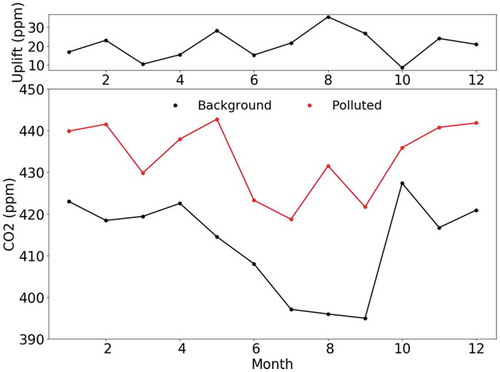
Figure 1 shows the time series of CO₂ concentrations in Xinglong during the period June 2016 to December 2017. The black dots are the filtered regional background values based on the robust extraction of the baseline signal. Figure 2 shows the monthly cycles of local sources and regional background CO₂ concentrations over a 12-month period and the upper panel shows their differences. Figure 2 shows that both the local sources and regional background CO₂ concentrations are low in summer, the season with the strongest photosynthetic uptake. The high regional background values in winter and early spring are due to positive biological fluxes (i.e., stronger plant respiration and weaker plant photosynthesis). The seasonal variations in Shangdianzi, which is also located in the Beijing–Tianjin–Hebei urban agglomeration on the North China Plain, are almost identical compared to that in Xinglong, with the lowest occurring in August and highest in March (Xia et al. 2016). In addition to weaker plant photosynthesis, CO₂ occupies 6.13% of the total emissions from straw burning in China in autumn (Cao et al. 2008), influencing the regional background signal in Xinglong in October. The increase in anthropogenic sources of CO₂ from domestic heating contributes to the higher CO₂ values during winter (Wang et al. 2010). The peak-to-trough value of the monthly regional background CO₂ concentration is 32.43 ± 10.95 ppm, proving the obvious seasonal variation in CO₂ in Xinglong station. Differences in the local sources and regional background CO₂ concentrations (upper panel in Figure 2) are large in summer and early autumn, reaching 21.63 ± 7.40, 35.56 ± 7.40, and 26.72 ± 7.40 ppm in July, August, and September, respectively (Fang et al. 2017). This indicates the strong influence of strong local sources in these two seasons. The relatively higher discrepancies in November and February also illustrate higher signals from local sources.

Figure 1. Time series of regional background (black) and non-background (gray) CO₂ concentrations in Xinglong.

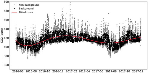
Figure 2. Monthly cycles of local sources and regional background CO₂ concentrations over a 12-month period. The upper panel shows the differences between the local sources and regional background CO₂ concentrations over a 12-month period. The lower panel shows the monthly cycles of local sources and regional background CO₂ concentrations over a 12-month period.

The least-squares method was used to fit the hourly average data of CO₂ to evaluate the diurnal cycles in the regional background CO₂ concentrations in different seasons that were not affected by linear trends. Figure 3 shows four diurnal cycles of CO₂.

Figure 3. Diurnal cycles of regional background concentrations of CO₂ by season.

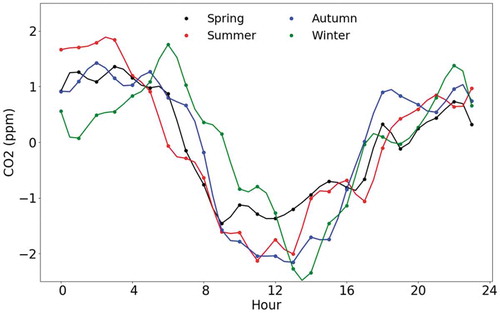
In general, the diurnal variations in CO₂ concentrations are significant in all seasons, with low values around 1000 to 1400 local time. This is because the stronger convection at noon mixes the near-ground high CO₂ concentrations with the low concentrations in the upper-level atmosphere. The weaker convective diffusion in the boundary layer limits the accumulation of CO₂ in the afternoon and high values usually occur at night. The peak-to-trough diurnal amplitudes are 2.82 ± 0.93, 3.97 ± 1.26, 3.58 ± 1.26, and 4.10 ± 1.06 ppm for spring, summer, autumn, and winter, respectively.

3.3. Influence of long-distance transport

Xinglong station is built on a relatively high hill and CO₂ concentrations are likely due to large-scale advection (Fang et al. 2016). We calculated the backward 72-h airflow trajectories arriving in the Xinglong area in all four seasons from May 2016 to December 2017 based on MeteoInfo software to analyze the long-distance transport contributing to CO₂ concentrations. Cluster analysis groups a large number of trajectories according to the horizontal movement velocity as well as the direction of the air masses and is applied to the analysis of the classification of different transportation (Shi et al. 2008). Based on the potential source contribution function (PSCF) algorithm, we calculated the quantitative contributions of potential areas for CO₂ in all four seasons in Xinglong (Begum et al. 2005).

Figure 4 shows the patterns of cluster analysis for the major 72-h backward trajectories in each season and the potential source contribution of CO₂ in Xinglong from May 2016 to December 2017. The numbers indicate the trajectory clustering type. The PSCF analysis is also shown in Figure 4 as a supplement to the backward trajectory analysis. The shading represents the probability distribution of emission sources. Table 1 shows the cluster analysis of trajectories, the average CO₂ concentrations in each cluster, and the regions the clusters run through.

Table 1. Statistical analysis of cluster trajectories, including trajectory numbers, ratios, average CO₂ concentrations in each cluster, and the regions each cluster runs through.

Season	Cluster	Trajectory number	Ratio	Average CO2 (ppm)	Through-regions
Spring	4	425	16.00%	418.68 ± 10.95	Tangshan and Tianjin in China
	2	714	26.88%	414.68 ± 8.49	Mongolia and Russia, Zhangjiakou in China
	6	436	16.42%	416.69 ± 9.18
	3	318	11.97%	411.18 ± 7.48
	1	506	19.05%	411.07 ± 5.65
	5	257	9.68%	413.26 ± 3.14	Mongolia, north of the station
Summer	1	1133	28.53%	407.30 ± 12.79	Beijing–Tianjin–Hebei and Shandong in China
	5	765	19.26%	409.85 ± 10.99
	4	322	8.11%	404.81 ± 14.05	Mongolia, Zhangjiakou in China
	2	1058	26.64%	401.43 ± 12.16
	3	693	17.45%	397.41 ± 11.03	Inner Mongolia and Chifeng in China
Autumn	1	680	17.33%	418.11 ± 13.20	Beijing–Tianjin–Hebei and Shandong in China
	3	686	17.48%	416.99 ± 12.52	Mongolia, Zhangjiakou and Wulumuqi in China
	4	1110	28.29%	417.05 ± 13.66
	5	844	21.51%	417.94 ± 13.49
	2	604	15.39%	408.38 ± 8.79	Mongolia
Winter	4	171	6.56%	423.84 ± 16.60	Mongolia and Russia, Zhangjiakou in Hebei
	2	516	19.79%	426.49 ± 12.99
	5	485	18.60%	425.26 ± 13.64
	1	526	20.17%	420.39 ± 12.28
	6	394	15.11%	412.54 ± 6.21	Mongolia
	3	516	19.79%	413.17 ± 5.61

Figure 4. Cluster analysis of 72-h backward trajectory and PSCF analysis of CO₂ in Xinglong from May 2016 to December 2017. The numbers indicate the trajectory clustering type and the color depth represents the probability distribution of the emission sources: the deeper the color, the greater the contribution.

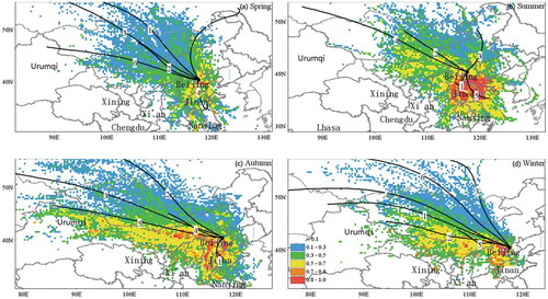
Most of the clusters in spring have pathways northwest of the station, where Mongolia, Russia and Zhangjiakou (in Hebei Province) are located. However, these regions are not expected to be a major contributor for clusters 1, 2, 3, and 6 (covering about 74.32%), which have lower mean CO₂ concentrations. Cluster 4 may transport anthropogenic emissions with relatively high CO₂ concentrations of 418.68 ± 10.95 ppm, from Tangshan and Tianjin. The slower speed of cluster 4 obstructs the dilution of strong emissions and hence CO₂ is accumulated before arriving in Xinglong.

The CO₂ concentrations in summer are more influenced by clusters 1 and 5 with higher CO₂ concentrations running through Beijing–Tianjin–Hebei and Shandong. Clusters 1 and 5 account for about 47.79%. Clusters 2 and 4, from Mongolia and Zhangjiakou, together with cluster 3 from the east of Inner Mongolia and Chifeng, are considered as relatively clean areas with lower CO₂ concentrations.

In autumn and winter, with the strong invasion of westerly wind, the west–north–west clusters through Mongolia, Urumqi, and Zhangjiakou all transport large amounts of CO₂. The urban agglomerations of Beijing–Tianjin–Hebei and Shandong also make a positive contribution to the concentrations of CO₂ in Xinglong in autumn, with the highest values of 418.11 ± 13.20 ppm for CO₂ carried by cluster 1. Although there is no obvious airflow from the Beijing–Tianjin–Hebei metropolitan area, the PSCF analysis shows that the anthropogenic emissions from these areas also make a large contribution to CO₂ concentrations in winter. Liu et al. (2009) also studied the relationship between the winds and the non-background CO₂ in Shangdianzi. They concluded that transport from Beijing–Tianjin–Hebei makes apparently positive contributions to the non-background CO₂ in Shangdianzi station, which acts similar to Xinglong station.

The PSCF (shaded areas in Figure 4) was also studied in addition to the cluster analysis of the 72-h backward trajectory. In spring, in addition to the regions determined from the cluster analysis, there is also a possible contribution from the cities in eastern Hebei Province. In summer, the potential sources of CO₂ are restricted to the south of the station, mainly in Hebei Province. The potential contributing areas in autumn for CO₂ are mainly located in two main directions: south to Henan Province and west-northwest to Inner Mongolia. Potential source areas for CO₂ in winter are concentrated in Beijing, north of Shanxi Province and west-northwest to Inner Mongolia.

4. Conclusions

This paper reports continuous measurements of atmospheric CO₂ in Xinglong from May 2016 to December 2017. The seasonal and diurnal variations in CO₂ concentrations, together with long-distance transport, are discussed.

The accuracy of the Picarro instrument in Xinglong meets the requirements of the WMO/GAW global network. The CO₂ concentrations are high in winter and low in summer. The seasonal variation in the regional background concentrations of CO₂ is mainly due to the photosynthesis and respiration of plants. Regional transport is another important factor. The airmass from southwest, south, and southeast of the station (e.g., from Beijing, Hebei Province, and Shandong Province) contributes to the high CO₂ concentrations, especially in summer. Transport from Inner Mongolia is another potential source for CO₂ in autumn and winter.

The diurnal patterns in CO₂ concentrations show relatively low values around 1000–1400 local time. For CO₂, the strong sunshine at noon results in stronger mixing of the near-surface atmosphere with that at higher levels, which dilutes the near-ground CO₂ concentrations. The more stable and lower boundary layer in the afternoon increases the concentrations of CO₂.

The measurements at Xinglong are made continuously and with regular calibration. With more collected data, we will be capable of analyzing the changes/trends of CO₂ in the near future. Meanwhile, instead of the regional background CO₂ measurements, we intend to study the relatively high and low CO₂ measurements and try to better understand the sources and sinks of CO₂ around Xinglong.

Acknowledgments

We express our great thanks to the staff at Xinglong station who contributed to the instrument’s maintenance at the station.

Disclosure statement

No potential conflict of interest was reported by the authors.

Supplementary material

Supplemental data for this article can be here.

Additional information

Funding

This research was funded by the National Key Research and Development Program  of China [grant numbers 2017YFB0504000 and 2017YFC1501701] and the National Natural Science Foundation of China [grant number 41575034].

References

- Andrews, A. E., J. D. Kofler, M. E. Trudeau, J. C. Williams, D. H. Neff, K. A. Masarie, D. Y. Chao, et al. 2014. “CO2, CO, and CH4 Measurements from Tall Towers in the NOAA Earth System Research Laboratory’s Global Greenhouse Gas Reference Network: Instrumentation, Uncertainty Analysis, and Recommendations for Future High-accuracy Greenhouse Gas Monitoring Efforts.” Atmos. Meas. Tech., 7: 647–687. doi:10.5194/amt-7-647-2014.
- Bakwin, P. S., P. P. Tans, D. F. Hurst, and C. L. Zhao. 1998. “Measurements of Carbon Dioxide on Very Tall Towers: Results of the NOAA/CMDL Program.” Tellus 50 (B): 401–415. doi:10.3402/tellusb.v50i5.16216.
- Begum, B. A., E. Kim, C. H. Jeong, D.-W. Lee, and P.K. Hopke. 2005. “Evaluation of the Potential Source Contribution Function Using the 2002 Quebec Forest Fire Episode.” Atmospheric Environment 39: 3719–3724. doi:10.1016/j.atmosenv.2005.03.008.
- Cao, G. L., X. Y. Zhang, Y. Q. Wang, and F. C. Zheng. 2008. “Estimation of Emissions from Field Burning of Crop Straw in China.” Chinese Science Bulletin 53 (5): 784–790. doi:10.1007/s11434-008-0145-4.
- Cheng, H. B., M. L. Wang, Y. X. Wen, and G. C. Wang. 2003. “Background Concentrations of Greenhouse Gases CO2, CH4, and N2O at Mt.waliguan and Xinglong Stations in China.” Journal of Applied Meteorology 14 (4): 402–409.
- Crosson, E. R. 2008. “A Cavity Ring-down Analyzer for Measuring Atmospheric Levels of Methane, Carbon Dioxide, and Water Vapor.” Applied Physics B 92 (3): 403–408. doi:10.1007/s00340-008-3135-y.
- Fang, S. X., L. X. Zhou, P. P. Tans, P. Ciais, M. Steinbacher, L. Xu, and T. Luan. 2014. “In Situ Measurement of Atmospheric CO2 at the Four WMO/GAW Stations in China.” Atmospheric Chemistry and Physics 14: 2541–2554. doi:10.5194/acp-14-2541-2014.
- Fang, S. X., P. P. Tans, B. Yao, T. Luan, Y. L. Wu, and D. J. Yu. 2017. “Study of Atmospheric CO2 and CH4 at Longfengshan WMO/GAW Regional Station: The Variations, Trends, Influence of Local Sources/sinks, and Transport.” Science China Earth Sciences 60: 1886–1895. doi:10.1007/s11430-016-9066-3.
- Fang, S. X., P. P. Tans, M. Steinbacher, L. X. Zhou, T. Luan, and Z. Li. 2016. “Observation of Atmospheric CO2 and CO at Shangri-La Station: Results from the Only Regional Station Located at Southwestern China.” Tellus B: Chemical and Physical Meteorology 68: 1–13. doi:10.3402/tellusb.v68.28506.
- Fang, S. X., T. Luan, G. Zhang, Y. L. Wu, and D. J. Yu. 2015. “The Determination of Regional CO2 Mole Fractions at the Longfengshan WMO/GAW Station: A Comparison of Four Data Filtering Approaches.” Atmospheric Environment 116 (10): 36–43. doi:10.1016/j.atmosenv.2015.05.059.
- IPCC-Intergovernmental Panel on Climate Change: Climate Change. 2013. The Physical Science Basis, Fifth Assessment Report of the Intergovernmental Panel on Climate Change. New York: Cambridge University Press.
- Liu, L. X., L. X. Zhou, X. C. Zhang, M. Wen, F. Zhang, B. Yao, and S. X. Fang. 2009. “Characteristics of Atmospheric CO2 Background Changes at Four National Level Stations in China.” Science China Earth Sciences 39: 222–228. doi:10.1007/s11430-009-0143-7.
- Peters, G. P., G. Marland, C. Le Quéré, T. Boden, J. G. Canadell, and M. R. Raupach. 2011. “Rapid Growth in CO2 Emissions after the 2008–2009 Global Financial Crisis.” Nature Climate Change 2: 2–4. doi:10.1038/nclimate1332.
- Ruckstuhl, A. F., S. Henne, S. Reimann, M. Steinbacher, M. K. Vollmer, S. O’Doherty, B. Buchmann, and C. Hueglin. 2012. “Robust Extraction of Baseline Signal of Atmospheric Trace Species Using Local Regression.” Atmospheric Measurement Techniques 5: 2613–2624. doi:10.5194/amt-5-2613-2012.
- Shi, C. E., Y. Q. Yao, P. Zhang, and M. Y. Qiu. 2008. “Transport Trajectory Classifying Of Pm10 in Hefei.” Plateau Meteorology (In Chinese) 6: 330–341.
- Thoning, K. W., P. P. Tans, and W. D. Komhyr. 1989. “Atmospheric Carbon Dioxide at Mauna Loa Observatory 2. Analysis of the NOAA GMCC Data, 1974–1985.” Journal of Geophysical Research Atmospheres 94 (D6): 8549–8565. doi:10.1029/JD094iD06p08549.
- Tuomas, L. 2007. “World Meteorological Organization Global Atmosphere Watch.” World Meteorological Organization, 145.
- Wang, Y., J. W. Munger, S. Xu, M. B. McElroy, J. Hao, C. P. Nielsen, and H. Ma. 2010. “CO2 and Its Correlation with CO at a Rural Site near Beijing: Implications for Combustion Efficiency in China.” Atmospheric Measurement Techniques 10: 8881–8897. doi:10.5194/acp-10-8881-2010.
- WMO data summary. 2017. “WMO World Data Centre for Greenhouse Gases (WDCGG) Data Summary: Greenhouse Gases and Other Atmospheric Gases, No. 41.” Japan Meteorological Agency. http://ds.data.jma.go.jp/gmd/wdcgg/pub/products/summary/sum41/sum41.pdf
- Wu, D., J. Y. Xin, Y. Sun, Y. S. Wang, and P. C. Wang. 2010. “Variation and Analysis of Background Concentration of Atmospheric Pollutants in North China during the 2008 Olympic Games.” Environmental Science 31 (5): 1130–1138.
- Xia, L. J., L. X. Zhou, L. X. Liu, and G. Zhang. 2016. “monitoring Atmospheric CO2 and δ13C(CO2) Background Levels at Shangdianzi Station in Beijing, China.” Environmental Science (In Chinese). 30: 2.
- Yan, K. P., L. X. Zhou, S. X. Fang, Y. X. Wen, B. Yao, F. Zhang, and L. X. Liu. 2011. “Flow and Method of Calibration Based on the New CO2 and CH4 Mixed Standard Gases.” Environmental Chemistry 37 (4): 511–516.
- Yver Kwok, C., O. Laurent, A. Guemri, C. Philippon, B. Wastine, C. W. Rella, C. Vuillemin, et al. 2015. “Comprehensive Laboratory and Field Testing of Cavity Ring-down Spectroscopy Analyzers Measuring H2O, CO2, CH4 and CO.” Atmospheric Measurement Techniques 8: 3867–3892. doi:10.5194/amt-8-3867-2015.
- Zhang, F., L. M. Zhou, and L. Xu. 2013. “Analysis of Variation of CH4 Concentration in the Atmosphere of Waliguan and Its Potential Source Regions.” Science China: Earth Sciences 56: 727–736. doi:10.1007/s11430-012-4577-y.
- Zhao, C. L., P. S. Bakwin, and P. P. Tans. 1997. “A Design for Unattended Monitoring of Carbon Dioxide on A Very Tall Tower.” Atmospheric and Oceanic Science Letters 14: 1139–1145. doi:10.1175/1520-0426(1997)014<1139:ADFUMO>2.0.CO;2.