Measuring and comparing in-situ CO₂ and CO profiles with satellite observations and model data

ABSTRACT

Accurate measurements of the vertical distribution of carbon dioxide (CO₂) in the atmosphere are critical to validate the vertical columns recorded by satellite and ground-based spectrometers and to estimate sources and sinks of CO₂. This work describes an in-situ air-sampler system (Aircore). Profiles of CO₂ and carbon monoxide (CO) were retrieved from two soundings of this system in Xilin Hot on 13 and 14 June 2018, and compared with observations from the Tropospheric Monitoring Instrument (TROPOMI), Orbiting Carbon Observatory-2 (OCO-2), and Copernicus Atmosphere Monitoring Service (CAMS). The column-averaged mixing ratio of CO (XCO) monitored by TROPOMI agreed well with that calculated from the in-situ CO profile, with a small mean difference of 5 ± 1.89 ppb. The column-averaged mixing ratio of CO₂ (XCO₂) monitored by OCO-2 also agreed well with that calculated from the in-situ CO₂ profile, with a slight bias of 0.4 ± 0.6 ppm. The OCO-2 a posteriori profile had an obvious bias compared with the in-situ CO₂ profile on 13 June, with an underestimation between 600 hPa and 250 hPa and an overestimation below 600 hPa. CAMS also had the same bias compared with the in-situ CO profile; however, CAMS agreed well with the in-situ CO profile on 14 June in the troposphere because a weak cold vortex passed Xilin Hot on 13 June and disappeared on 14 June. In the stratosphere, there were significant biases in the vertical degradation. The striking agreement between the column-averaged mixing ratios and the differences in the vertical distribution suggests new exciting applications for the profile product.

Graphical abstract

摘要

准确测量CO₂在大气中的垂直分布对于验证卫星和地基光谱仪及估计CO₂源、汇至关重要。本文描述了一种原位大气采样系统（aircore）。我们利用这套系统在内蒙古锡林浩特地区于2018年6月13日和14日获取了CO₂和CO廓线并与对流层监测仪（TROPOMI），轨道碳观测（OCO-2）和哥白尼大气监测服务（CAMS）比较。TROPOMI 监测的CO柱总浓度（XCO）与原位测量CO廓线计算的XCO一致，平均偏差为5±1.89 ppb。OCO-2监测的CO₂柱总浓度与原位测量廓线所得结果一致，平均偏差为.0.4±0.6ppm。6月13日，OCO-2后验廓线与原位测量廓线有明显偏差，OCO-2低估了250 hPa和600 hPa高度间的CO₂浓度，高估了600 hPa高度以下的CO₂浓度。CAMS的CO廓线与原位测量廓线在6月13日的偏差与OCO-2相似，但是在6月14日偏差较小。因为6月13日，一个弱的低压环流经过锡林浩特地区并于6月14日消失。在平流层，它们的偏差都很显著。柱总浓度的一致性和垂直分布的明显偏差说明这套廓线产品具有进一步的科学应用价值。

KEYWORDS:

• Aircore
• greenhouse gas
• profile

关键词:

• 长管下投采样
• 温室气体
• 廓线

1. Introduction

Understanding the global atmospheric budget of the carbon dioxide (CO₂) emitted by human activities is essential to control existing levels and predicting future changes. To this end, several methods have been developed to improve the monitoring of atmospheric CO₂. Many World Meteorological Organization surface-based stations have been used to measure its atmospheric concentration. However, these ground-based stations are still too sparse to fully determine the surface flux at the regional scale. Several space-based instruments have therefore been launched to measure the column density of greenhouse gases globally, such as the Atmospheric Infrared Sounder (Crevoisier, Chedin, and Scott 2003), Scanning Imaging Absorption Spectrometer for Atmospheric Cartography (Frankenberg et al. 2011), Tropospheric Emission Spectrometer (Worden et al. 2012), Greenhouse Gases Observing Satellite (Butz et al. 2011), Orbiting Carbon Observatory-2 (OCO-2) (Hammerling, Michalak, and Randolph Kawa 2012), and the Chinese carbon satellite (TanSat) (Liu et al. 2018). However, satellite measurements need additional information regarding the vertical distribution of greenhouse gases to determine the a posteriori column integrals and validate their monitoring results from space. The Total Column Carbon Observing Network (TCCON), which is a cluster of ground-based Fourier transform spectrometers (Petersen et al. 2008; Warneke et al. 2005), has been established to validate the measurements made by satellites.

Due to the limited vertical profile information, both space- and ground-based spectrometers must determine the vertical distribution of trace gases to constrain the retrieved column (Rodgers 2000). Additionally, atmospheric chemistry transport models require accurate vertical distributions of trace gases to estimate regional fluxes (Lamarque et al. 2013).

Aircraft-based equipment can accurately measure the CO₂ concentration at specific heights. However, measurements cannot be made at altitudes higher than 15 km. Stratospheric balloons can compensate for the missing values from around 15–35 km. Profiles derived from stratospheric balloons are valuable because they do not require as much extrapolation and interpolation of measurements as profiles obtained above the aircraft ceiling, reducing the uncertainty in the column integral.

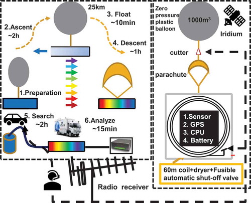
Aircore, which was first proposed and designed by Pieter Tans (2009) at the National Oceanic and Atmospheric Administration (NOAA) Earth System Research Laboratory, is an innovative atmospheric sampling system. It consists of a long coil of stainless steel tubing. The top left panel of Figure 1 presents the basic Aircore concept. Aircore ascends on a helium balloon and collects samples of the surrounding atmosphere during a parachute-controlled descent. Sample collection commences after separation from the balloon (up to 25 km). An Aircore sample can be analyzed using a continuous trace gas analyzer in a mobile laboratory. The long tube and short time between sampling and analysis minimize mixing inside the tubing, so that each Aircore sample can provide up to 100 measurements of CO₂, methane (CH₄) and CO between the altitude reached and the ground. Aircore can capture a continuous profile with low cost at vertical resolutions from 500 m to 5 km. High resolution using a lighter Aircore device, especially in the upper troposphere–lower stratosphere (UTLS) region, has been established by NOAA, Groningen University, and Goethe University Frankfurt. Andersen et al. (2018) used an unmanned aerial vehicle to carry the Aircore, and Mrozek et al. (2016) designed an air sub-sampler that can collect and preserve the sample collected from the Aircore for the analysis of isotopes.

Figure 1. Left: the Aircore sampling process. Right: the Aircore system.

Based on the Aircore design, a similar sample system was developed in China through a collaborative effort by the Meteorological Observation Center and Institute of Atmospheric Physics. Two CO₂ and CO profiles were retrieved from launches on June 2018 in Inner Mongolia. In this paper, we describe the design of the Chinese Aircore system and compare the profiles obtained with model simulations and satellite measurements.

The paper is structured as follows: Section 2 describes the newly developed Aircore system, including sample theory and data processing. Section 3 provides details of the field campaign. Section 4 presents the profiles and a comparison with model and satellite measurements. Finally, section 5 provides a summary and conclusions.

2. Data acquisition

2.1 The Aircore device

The Aircore device consists of three subsystems: sounding, control and communication, and mobile analysis. The right-hand panel of Figure 1 presents the sounding part. The main payload is a 60-m long, 304-grade stainless steel tube treated with a sulfinert coating (Restek, Inc., State College, PA, USA). Two 30-m long tubes, with an outer diameter of 0.635 cm (wall thickness of 0.089 cm) and 0.3175 cm (wall thickness of 0.0711 cm), are used to obtain a high resolution in the UTLS region. A short stainless steel tube filled with fresh magnesium perchlorate powder is attached to one end of the Aircore to ensure that no moisture enters the tubing during testing and sampling. The fusible automatic shut-off valve can be closed automatically or by a control signal when the pressure change is less than 10 hPa after landing. The overall weight is around 5 kg. Unlike other Aircore systems, we use a zero-pressure balloon as a platform. It has a vent to the atmosphere at the bottom. The balloon is only partially filled on the ground. As the balloon rises, the gas bubble expands to fill out the balloon from the top downward. When the gas bubble expands to completely fill the balloon, excess gas exhausts through the vent at the bottom. At this point, the ascent stops, and the balloon hovers at a constant altitude. The sounding hovers for tens of minutes to stabilize, and then instructions are sent to the cutter. The payload separates from the balloon and the parachute opens to avoid a fast descent that would generate large differences between the pressure inside and outside the tube. For the control and communication sub-system, a radio and iridium/GPS collar are used to retrieve the position of the Aircore during the flight and after landing.

In the mobile analysis sub-system, high-purity CO gas is used to push the collected gas through the device and obtain the sample. One end of the tube is linked to the high-purity CO gas tank and the other end is linked to a PICARRO G2301 gas analyzer (Picarro, Santa Clara, CA, USA). The main difference between this device and the existing Aircore is that the analysis system is mobile, and does not require taking the sample tube back to the laboratory. The time between sampling and analysis is approximately four hours. This ensures that the air in the tube only diffuses a short distance and the resolution is relatively high. For more detail regarding the analysis system, please refer to Miao et al. (2019).

2.2 Field campaign in Inner Mongolia

Two soundings were launched at Xilin Hot, Inner Mongolia (44°N, 116°E, 1004 m MSL) on 13 and 14 June 2018, referred to as flights 1 and 2. The main land use over Inner Mongolia is grassland, although no grass was growing at the launch site during the Aircore campaign. The two flights were launched at around 07:00 (UTC+8), just after radiosondes were released from the local weather station, which were used to predict the trajectory of the Aircore. The Aircore system hovered at an altitude of ~24 km altitude for 1 h and 10 min for flights 1 and 2, respectively. In flight 1, the valve was manually closed so the heating that occurred during this period resulted in the loss of a fraction of the profile equivalent to the air sampled from 820 to 890 hPa. TROPOMI and OCO-2 both passed by Xinlin Hot on 13 June.

2.3 Data processing

After the analysis, we obtained a trace gas mole fraction time series. To obtain a trace gas profile (e.g. CO₂) we needed to convert the time axis to an altitude axis. The critical orifice set the flow rate during analysis to 40 standard cubic centimeter minutes (sccm) and controlled the settings of the Picarro analysis cell to ensure that the same number of moles were analyzed at every time step. The number of moles flowing through the analyzer increased linearly with time. The number of moles at any given time was:

(1) $n_i=n_{\mathrm{m}\mathrm{a}\mathrm{x}}\frac{t_i}{t_{\mathrm{t}\mathrm{o}\mathrm{t}\mathrm{a}\mathrm{l}}},$(1)

where $t_{\mathrm{t}\mathrm{o}\mathrm{t}\mathrm{a}\mathrm{l}}$ is the total time of the analysis, $n_i$ is mole of sample analyzed at the time step i, $t_i$ is the total time of the analysis at the time step i, $n_{\mathrm{m}\mathrm{a}\mathrm{x}}$ is the maximum mole of sample when finishing analyses.

Because we logged the temperature of the tube and ambient pressure, we could calculate the mole fraction at each altitude based on the ideal gas law. The maximum mole fraction occurred when the Aircore reached the Earth’s surface:

(2) $\frac{t_i}{t_{\mathrm{t}\mathrm{o}\mathrm{t}\mathrm{a}\mathrm{l}}}=\frac{n_i}{n_{\mathrm{m}\mathrm{a}\mathrm{x}}}=\frac{P_i{T}_{\mathrm{g}\mathrm{r}\mathrm{o}\mathrm{u}\mathrm{n}\mathrm{d}}}{T_i{P}_{\mathrm{g}\mathrm{r}\mathrm{o}\mathrm{u}\mathrm{n}\mathrm{d}}},$(2)

where $P_i$ and $T_i$ are the ambient pressure and temperature of the tube at specific altitudes, respectively, and $P_{\mathrm{g}\mathrm{r}\mathrm{o}\mathrm{u}\mathrm{n}\mathrm{d}}$ and $T_{\mathrm{g}\mathrm{r}\mathrm{o}\mathrm{u}\mathrm{n}\mathrm{d}}$ are the pressure and temperature of the tube at the surface.

3. Results

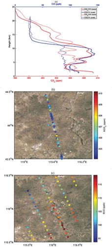
Figure 2 presents the measured mole fractions of CO and CO₂ against altitude for the two flights. Each profile comprises about 430 points on the vertical axis. Because the fill gas remaining in the coil was high-purity CO, we only retrieved the CO profile from 2 to 20 km.

Figure 2. (a) Red lines represent CO₂ and blue lines represent CO. Solid lines represent 13 June and dotted lines represent 14 June. The y-axis is the height above mean sea level (km). XCO₂ and XCO along the trajectory of (b) OCO-2 and (c) TROPOMI. The circles represent satellite observations and the pentagrams represent Aircore measurements. The map is taken from Google Earth.

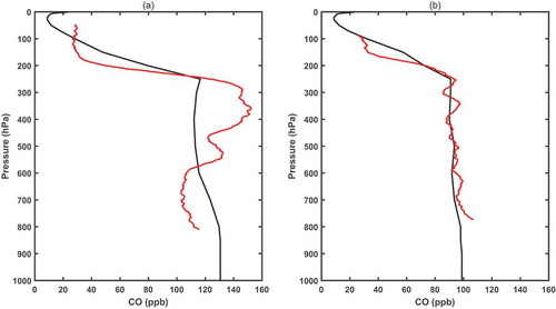
The Copernicus Atmosphere Monitoring Service (CAMS) has been providing global forecasts and analysis of atmospheric composition on a daily basis at ECMWF for nearly a decade, with applications in air quality and monitoring of long-lived greenhouse gases. Figure 3 compares the Aircore and CAMS CO profiles. In the stratosphere, the differences were reasonably large on both days. The mean difference was −16.8 ppb for 13 June, with a standard deviation of 13.68 ppb, while it was −4.82 ppb for 14 June, with a standard deviation of 13.19 ppb. In the troposphere, the difference between CAMS and Aircore was small on 14 June, with mean values of 1.71 and 3.03 ppb, respectively. The difference was larger on 13 June, with CAMS overestimating in the lower troposphere and underestimating in the upper troposphere. The mean difference was 21.55 ppb, with a standard deviation of 13.42 ppb in the lower troposphere, while it was −15.5 ppb, with a standard deviation of 5.48 ppb, in the upper troposphere. This is because a weak cold vortex passed Xilin Hot on 13 June and disappeared on 14 June. The weather conditions resulted in obvious differences in the comparison between CAMS and Aircore.

Figure 3. Comparison of Aircore CO vertical profiles (red line) with co-located simulation values from CAMS (black line) at the landing coordinates on (a) 13 June and (b) 14 June.

TROPOMI passed by Xilin Hot on 13 June. We selected the area centered within 0.5° of Xilin Hot (Figure 2(c)). The column-averaged CO mixing ratio (XCO) was 118 ppb, with a standard deviation of 1.89 ppb, while the XCO derived from Aircore was 113 ppb, and that from CAMS was 105 ppb (Table 1). There was good agreement between TROPOMI and Aircore. Unfortunately, there were no TROPOMI data on 14 June around Xilin Hot. The XCO on 14 June was 84.6 ppb from Aircore and 83.9 ppb from CAMS. They agreed well with each other on 14 June. Borsdorff et al. (2018) also reported that TROPOMI was well correlated with CAMS. The mean difference between TROPOMI and CAMS was 3.2% ± 5.5%. Aircore was, therefore, considered to provide credible in-situ measurements.

Table 1. Comparison of XCO₂ and XCO among satellites (OCO-2 and TROPOMI), CAMS, and Aircore.

	CO2	CO
Satellite	405.6 ppm ± 0.6 ppm(OCO-2)	118 ppb ± 1.89 ppb(TROPOMI)
CAMS	\	105 ppb
Aircore	406 ppm	113 ppb

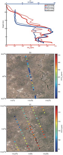
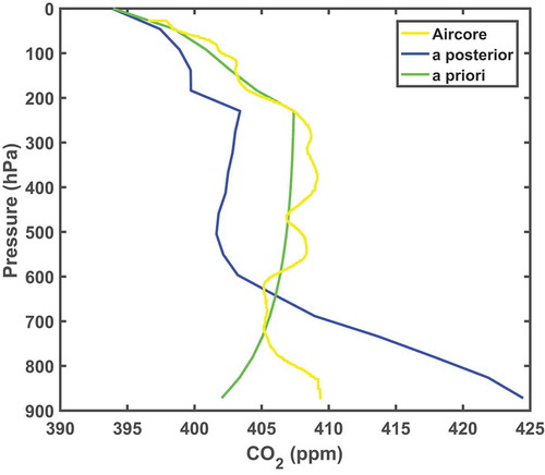
In addition to CO, we also validated the column-averaged CO₂ mixing ratio (XCO₂) calculated from Aircore with OCO-2 observations. Fortunately, OCO-2 passed by Xilin Hot on 13 June and the area selected for the comparison was the same as that used for the TROPOMI comparison. After filtering the data using a threshold level ≥3, the XCO₂ measured by OCO-2 was 405.6 ± 0.6 ppm and the XCO₂ derived from Aircore was 406 ppm (Table 1). Aircore, therefore, agreed well with OCO-2. The XCO₂ retrieved from OCO-2 was also compared with TCCON, and the absolute median differences were less than 0.4 ppm (Wunch et al. 2011). However, the vertical profile of CO₂ differed between OCO-2 and Aircore. Figure 4 presents the a priori and a posteriori vertical profiles of CO₂ from the OCO-2 compared with the vertical profile obtained from Aircore. As shown in Figure 4, the a posteriori CO₂ vertical profile reflected the overall features of depleted low-altitude (below 600 hPa) and enhanced high-altitude CO₂, but the vertical gradient compared with Aircore was very different. Below 600 hPa, OCO-2 overestimated the CO₂, with a mean difference of −3.5 ± 2 ppm. Above 600 hPa, OCO-2 underestimated the CO₂, with a mean difference of 2.3 ± 1.2 ppm. The difference was greatest (3.98 ppm) at 376 hPa, where the enhanced CO₂ value in the free troposphere was measured by Aircore. Overall, in terms of XCO₂, OCO-2 agreed well with Aircore, but for the vertical distribution, OCO-2 had a 3 ppm mean difference compared with Aircore.

Figure 4. The a priori (green) and a posteriori (blue) vertical CO₂ profiles from OCO-2, and Aircore vertical CO₂ profile (yellow), on 13 June.

4. Conclusions

We developed a prototype Aircore-like system (Tans 2009; Karion et al. 2010) consisting of a 60-m tube, which was a combination of a 30-m-long with an outer diameter of 0.3175 cm and a wall thickness of 0.089 cm tube and a 30-m-long with an outer diameter of 0.635 cm and a wall thickness of 0.0711 cm tube, to improve the resolution in the UTLS region (Membrive et al. 2017). Instead of a rubber balloon, we used a zero-pressure plastic balloon that would not burst at the top of the troposphere and could, therefore, remain suspended for several minutes.

We conducted an Aircore campaign in Xilin Hot on 13 June and 14 June. We calculated the column-averaged mixing ratios from CO and CO₂ profiles and compared them with TROPOMI and OCO-2. We found good agreement between Aircore and TROPOMI, with a small mean difference of 5 ± 1.89 ppb. The XCO₂ derived from Aircore and OCO-2 was almost the same (OCO-2 was 405.6 ± 0.6 ppm and Aircore was 405 ppm), but their profiles were different. OCO-2 overestimated the CO₂ below 600 hPa, with a mean difference of −3.5 ± 2 ppm, and underestimated the CO₂ above 600 hPa, with a mean difference of 2.3 ± 1.2 ppm.

This is the first Aircore campaign in China, although the Aircore design was comparable with the devices used in other countries, e.g. the Netherlands, Germany, and France. We will improve our Aircore device to attain a higher resolution, especially in the UTLS, during an Aircore campaign in November 2018. We will simultaneously measure the mole fraction of more trace gases (CH₄, O₃, and N₂O). We will also use the environmental monitoring system EM27 which is an open path Fourier Transform infrared spectrometer to evaluate the Aircore retrieval and test the improvements in the instruments in more detail.

However, the results already obtained suggest that our current Aircore data product is satisfactory and can be used to support future goals, such as better understanding stratosphere–troposphere exchange processes under different weather systems and evaluating CO₂ flux inversion models.

Disclosure statement

No potential conflict of interest was reported by the authors.

Additional information

Funding

This study was supported by the Strategic Priority Research Program of the Chinese Academy of Sciences [grant number XDA17010102], the National Natural Science Foundation of China [grant number 41875043], and the Key Research Program of the Chinese Academy of Sciences [grant number ZDRW-ZS-2019-1].

References

- Andersen, T., B. Scheeren, W. Peters, and H. L. Chen. 2018. “A UAV-based Active AirCore System for Measurements of Greenhouse Gases.” Atmospheric Measurement Techniques 11 (5): 2683–2699. doi:10.5194/amt-11-2683-2018.
- Borsdorff, T., J. Aan de Brugh, H. Hu, I. Aben, O. Hasekamp, and J. Landgraf. 2018. “Measuring Carbon Monoxide with TROPOMI: First Results and a Comparison with ECMWF-IFS Analysis Data.” Geophysical Research Letters 45 (6): 2826–2832. doi:10.1002/2018gl077045.
- Butz, A., S. Guerlet, O. Hasekamp, D. Schepers, A. Galli, I. Aben, C. Frankenberg, et al. 2011. “Toward Accurate CO2 and CH4 Observations from GOSAT.” Geophysical Research Letters 38. doi:10.1029/2011gl047888.
- Crevoisier, C., A. Chedin, and N. A. Scott. 2003. “AIRS Channel Selection for CO2 and Other Trace-gas Retrievals.” Quarterly Journal of the Royal Meteorological Society 129 (593): 2719–2740. doi:10.1256/qj.02.180.
- Frankenberg, C., I. Aben, P. Bergamaschi, E. J. Dlugokencky, R. van Hees, S. Houweling, P. van der Meer, R. Snel, and P. Tol. 2011. “Global Column-averaged Methane Mixing Ratios from 2003 to 2009 as Derived from SCIAMACHY: Trends and Variability.” Journal of Geophysical Research-Atmospheres 116. doi:10.1029/2010jd014849.
- Hammerling, D. M., A. M. Michalak, and S. Randolph Kawa. 2012. “Mapping of CO2 at High Spatiotemporal Resolution Using Satellite Observations: Global Distributions from OCO-2.” Journal of Geophysical Research-Atmospheres 117. doi:10.1029/2011jd017015.
- Karion, A., C. Sweeney, P. Tans, and T. Newberger. 2010. “AirCore: An Innovative Atmospheric Sampling System.” Journal of Atmospheric and Oceanic Technology 27 (11): 1839–1853. doi:10.1175/2010jtecha1448.1.
- Lamarque, J. F., D. T. Shindell, B. Josse, P. J. Young, I. Cionni, V. Eyring, D. Bergmann, et al. 2013. “The Atmospheric Chemistry and Climate Model Intercomparison Project (ACCMIP): Overview and Description of Models, Simulations and Climate Diagnostics.” Geoscientific Model Development 6 (1): 179–206. doi:10.5194/gmd-6-179-2013.
- Liu, Y., J. Wang, L. Yao, X. Chen, Z. Cai, D. Yang, Z. Yin, et al. 2018. “The TanSat Mission: Preliminary Global Observations.” Science Bulletin 63 (18): 1200–1207. doi:10.1016/j.scib.2018.08.004.
- Membrive, O., C. Crevoisier, C. Sweeney, F. Danis, A. Hertzog, A. Engel, H. Bonisch, and L. Picon. 2017. “AirCore-HR: A High-resolution Column Sampling to Enhance the Vertical Description of CH4 and CO2.” Atmospheric Measurement Techniques 10 (6): 2163–2181. doi:10.5194/amt-10-2163-2017.
- Miao, L., F. Shuangxi, Y. Liu, B. Yao, W. Yong, M. Qianli, Y. You, and G. Mingrui. 2019. “Vertical Gradient Sampling Analysis Technology Based on Air Pressure Height Difference and Vertical Profile Observation of Carbon Dioxide.” China Environmental Science. in press.
- Mrozek, D. J., C. van der Veen, M. E. G. Hofmann, H. Chen, R. Kivi, P. Heikkinen, and T. Rockmann. 2016. “Stratospheric Air Sub-sampler (SAS) and Its Application to Analysis of Delta O-17(CO2) from Small Air Samples Collected with an AirCore.” Atmospheric Measurement Techniques 9 (11): 5607–5620. doi:10.5194/amt-9-5607-2016.
- Petersen, A. K., T. Warneke, M. G. Lawrence, J. Notholt, and O. Schrems. 2008. “First Ground-based FTIR Observations of the Seasonal Variation of Carbon Monoxide in the Tropics.” Geophysical Research Letters 35 (3). doi:10.1029/2007gl031393.
- Rodgers, C. D. 2000. Inverse Methods for Atmospheric Sounding: Theory and Practice, World Scientific, 238. Singapore: World Scientific.
- Tans, P. P., 2009. “System and method for providing vertical profile measurements of atmospheric gases.” U.S. Patent 7,597,014, filed 15 August 2006, and issued 6 October 2009.3.
- Warneke, T., R. de Beek, M. Buchwitz, J. Notholt, A. Schulz, V. Velazco, and O. Schrems. 2005. “Shipborne Solar Absorption Measurements of CO2, CH4, N2O and CO and Comparison with SCIAMACHY WFM-DOAS Retrievals.” Atmospheric Chemistry and Physics 5: 2029–2034. doi:10.5194/acp-5-2029-2005.
- Worden, J., S. Kulawik, C. Frankenberg, V. Payne, K. Bowman, K. Cady-Peirara, K. Wecht, J. E. Lee, and D. Noone. 2012. “Profiles of CH4, HDO, H2O, and N2O with Improved Lower Tropospheric Vertical Resolution from Aura TES Radiances.” Atmospheric Measurement Techniques 5 (2): 397–411. doi:10.5194/amt-5-397-2012.
- Wunch, D., P. O. Wennberg, G. C. Toon, B. J. Connor, B. Fisher, G. B. Osterman, C. Frankenberg, et al. 2011. “A Method for Evaluating Bias in Global Measurements of CO2 Total Columns from Space.” Atmospheric Chemistry and Physics 11 (23): 12317–12337. doi:10.5194/acp-11-12317-2011.