Numerical simulation of an extreme haze pollution event over the North China Plain based on initial and boundary condition ensembles

ABSTRACT

The North China Plain often suffers heavy haze pollution events in the cold season due to the rapid industrial development and urbanization in recent decades. In the winter of 2015, the megacity cluster of Beijing–Tianjin–Hebei experienced a seven-day extreme haze pollution episode with peak PM_2.5 (particulate matter (PM) with an aerodynamic diameter ≤ 2.5 μm) concentration of 727 μg m⁻³. Considering the influence of meteorological conditions on pollutant evolution, the effects of varying initial conditions and lateral boundary conditions (LBCs) of the WRF-Chem model on PM_2.5 concentration variation were investigated through ensemble methods. A control run (CTRL) and three groups of ensemble experiments (INDE, BDDE, INBDDE) were carried out based on different initial conditions and LBCs derived from ERA5 reanalysis data and its 10 ensemble members. The CTRL run reproduced the meteorological conditions and the overall life cycle of the haze event reasonably well, but failed to capture the intense oscillation of the instantaneous PM_2.5 concentration. However, the ensemble forecasting showed a considerable advantage to some extent. Compared with the CTRL run, the root-mean-square error (RMSE) of PM_2.5 concentration decreased by 4.33%, 6.91%, and 8.44% in INDE, BDDE and INBDDE, respectively, and the RMSE decreases of wind direction (−5.19%, −8.89% and −9.61%) were the dominant reason for the improvement of PM_2.5 concentration in the three ensemble experiments. Based on this case, the ensemble scheme seems an effective method to improve the prediction skill of wind direction and PM_2.5 concentration by using the WRF-Chem model.

GRAPHICAL ABSTRACT

摘要

目前，强霾事件中气象场的不确定性对PM_2.5浓度分布影响的研究较少。本文利用ECMWF发布的最新一代再分析资料ERA5在WRF-Chem模式下针对2015年冬季京津冀地区一次强霾事件设计了大气初值和侧边界条件的集合模拟试验。试验结果表明：三组不同集合方案分别使得PM_2.5浓度均方根误差（RMSE）相对于参照试验降低了4.33%、6.91%和8.44%，同时扰动初值和侧边界值的集合试验有效提高了模拟结果的准确性，这是因为集合方案有效改进了近地面风向模拟。以10米风向为例，RMSE分别降低了5.19%、8.89%和9.61%。在本个例中，集合模拟方案最高可使得重霾期间因气象场的不确定性引起的PM_2.5浓度模拟误差降低32%以上。

KEYWORDS:

• Haze pollution
• PM_2.5
• WRF-Chem
• initial and lateral boundary conditions
• ensemble forecasting

关键词:

• 霾污染
• PM_2.5
• WRF-Chem
• 初值条件
• 侧边界值条件
• 集合预报

1. Introduction

With the rapid industrial development and urbanization that has taken place in eastern China during the last several decades, the frequency and intensity of haze pollution have also been increasing— especially in the megacity cluster of Beijing–Tianjin–Hebei (BTH) (Zheng 2013; Cai et al. 2017a; Wu, Ding, and Liu 2017; Li et al. 2018). BTH is located in the North China Plain region, which is one of the most severe haze pollution regions in China (Quan et al. 2014; Yang et al. 2015). In January 2013, a total of five heavy haze pollution episodes were recorded over this region, with the highest hourly PM_2.5 concentration reaching approximately 1000 μg m⁻³ (Ji et al. 2014). Such a sharp decline in air quality greatly threatens human health and traffic safety (Xu, Chen, and Ye 2014).

In view of the frequent occurrence and seriousness of haze pollution events, accurate air quality prediction is demanding. Numerical simulation experiment of past haze events is a good way for achieving an understanding of the formation mechanisms, regional transportation and source apportionment of air pollution (Yang et al. 2015; Li et al. 2017; Wang et al. 2018). However, due to the highly nonlinear nature of the atmosphere and chemical substances, it is still a challenge to accurately predict severe haze events, even with state-of-the-art numerical models (Mallet, Stoltz, and Mauricette 2009; Zhang et al. 2012; Tuccella et al. 2012; Zhang et al. 2017). Ensemble-based forecasting has been investigated to improve the predictability of PM_2.5 concentration. For example, Cai et al. (2017b) carried out PM_2.5 ensemble forecasting experiments over Tianjin using the Weather Research and Forecasting model coupled to chemistry (WRF-Chem) based on various boundary layer schemes, which reduced the relative error and root-mean-square error (RMSE) of PM_2.5 concentration. Wang et al. (2009) constructed a multi-model ensemble operational forecasting system based on NAQPMS (Nested Air Quality Prediction Modeling System), CMAQ (Community Multiscale Air Quality), CAM_X (Comprehensive Air Quality Model with Extensions) and other models, and the correlation coefficient of daily mean PM₁₀ (PM with an aerodynamic diameter ≤ 10.0 μm) during the Beijing Olympic Games exceeded 0.7. Besides, the weighted integration method using different model components was found to be better than the arithmetic average result. Multi-model ensemble forecasting with the linear regression method, as reported by Huang et al. (2015), can reduce the uncertainty of PM₁₀ forecasts and improve the skill in predicting pollution episodes over the Beijing area.

The dominant multi-model ensemble or varying the model physics parameterization scheme ensemble in air quality forecasting aims to reduce the uncertainties caused by physical and chemical parameterizations and numerical calculation methods (Žabkar, Koračin, and Rakovec 2013; Petersen et al. 2018; Crippa et al. 2019). In fact, a lack of consideration for emission sources and meteorological conditions can also lead to large uncertainties in air quality simulation (Tang et al. 2010). However, few studies have investigated the effects of variations in meteorological fields on the simulation or prediction of PM_2.5 concentration. Therefore, the purpose of this study was to explore the effects of varying the initial and lateral boundary values of meteorological fields on the generation and transmission of PM_2.5 through ensemble runs with the WRF-Chem model, and to evaluate whether the ensemble experiments can effectively improve the simulation of PM_2.5 concentration in regional air quality models. An extreme haze pollution event in 2015 was selected as a typical case to carry out the study.

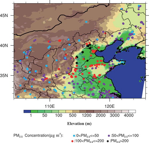
The North China Plain suffered a series of serious haze pollution events in winter 2015 (Zhang et al. 2017). From 26 November to 2 December, the megacity cluster of Beijing–Tianjin–Hebei (BTH) endured an extreme regional haze pollution event. Most of the hourly mean PM_2.5 concentrations during this haze episode exceeded 100 μg m⁻³, and were even higher than 200 μg m⁻³ in Beijing and central and southern Hebei (Figure 1). The observed peak concentration of PM_2.5 reached 727 μg m⁻³ on 30 November in the city of Baoding, and it was higher than 500 μg m⁻³ in Beijing throughout most of the day on 1 December. Because of the severity of this event, many studies on its formation and evolution processes have been carried out, as well as the associated regional transportation and source apportionment (Sun et al. 2016; Li et al. 2017). Li et al. (2017) found that this event can be divided into four stages: the slow formation stage (27–28 November); the peak-sustaining stage, except in Beijing (29–30 November); the rapidly increasing stage in Beijing (1 December); and the clearance stage (2 December). In our study, the focus was on an evaluation of ensemble simulation results.

Figure 1. The model domain with elevation (shaded; units: m). Blue, purple, red, and black dots denote the observed hourly averaged PM_2.5 concentration (units: μg m⁻³) during 26 November to 2 December. The abbreviations BJ, TJ, BD, CZ, SJZ, HS, XT, and HD denote the eight cities as defined in the text.

The data, model configuration, and experiment design used in this study are described in section 2. A basic model verification and detailed analysis of the ensemble simulation results are presented in section 3. A summary and concluding remarks are given in the final section.

2. Data and experiment design

2.1 Observation data

Hourly surface environmental monitoring data provided by the Ministry of Ecological Environment (http://106.37.208.233:20035) were used, including PM_2.5, SO₂, NO₂, and CO concentrations. Conventional in-situ meteorological observation data (e.g., 2 m temperature, relative humidity, 10 m wind speed and direction) were derived from the China Meteorological Administration (http://data.cma.cn/). Based on the PM_2.5 concentration spatial distribution, eight cities were selected for detailed analysis (shown in Figure 1): Beijing (BJ), Tianjin (TJ), Shijiazhuang (SJZ), Handan (HD), Baoding (BD), Cangzhou (CZ), Hengshui (HS) and Xingtai (XT).

2.2 Model configuration and experiment design

In this study, the WRF-Chem model, version 3.9.1.1 (Grell et al. 2005; Skamarock et al. 2008; Peckham et al. 2011; Powers et al. 2016) was adopted to simulate the heavy haze pollution event. Considering the influence of meteorological conditions on pollutant evolution, the effects of varying the initial conditions and lateral boundary conditions (LBCs) of WRF-Chem on the variation in PM_2.5 concentration were investigated through ensemble methods. We carried out a control run (CTRL) and three groups of ensemble forecasting experiments based on different atmospheric initial conditions and LBCs. All of the experiments shared the same physical and chemical parameterization schemes: the Morrison double-moment microphysics scheme, RRTMG short- and longwave radiation schemes, Noah land surface model, Yonsei University planetary boundary layer scheme, Grell–Freitas cumulus parameterization scheme, CBMZ chemical mechanism and MOSAIC using eight sectional aerosol bins including some aqueous reactions, and Fast-J photolysis. Besides, we opened sensible and latent heat fluxes on the ground and the radiation feedback mechanism for clouds in the physical process. The dry and wet deposition of aerosols and the direct effect between aerosols and clouds have been considered in the chemical process (Chapman et al. 2009). A 0.25° × 0.25° spatial resolution of anthropogenic emissions (monthly in 2012) was used as the chemical fields to initialize the WRF-Chem model, which was provided by the MEIC (Multi-resolution Emissions Inventory for China) group of Tsinghua University (http://www.meicmodel.org/) (Li et al. 2014; Liu et al. 2015; Cheng et al. 2016). Figure 1 shows the model domain with a grid size of 9 km. There were 30 σ-levels in the vertical direction and the model top was set at 50 hPa.

We used the latest released fifth-generation European Centre for Medium-Range Weather Forecasts (ECMWF) atmospheric reanalysis of the global climate (i.e., ERA5) as the model initial conditions and LBCs. The ERA5 dataset is composed of a 31 km high-resolution forecast (HRES) and a 62 km reduced-resolution 10-member 4D-Var ensemble of data assimilation (EDA) in CY41R2 of ECMWF’s Integrated Forecast System (IFS) . In our study, both HRES and the 10 EDA members were pre-interpolated to a regular 0.25° × 0.25° latitude/longitude grid with 137 hybrid sigma/pressure (model) levels in the vertical direction. HRES and the 10 EDA members are available hourly and every three hours, respectively. It was found that the meteorological forcing variables do show distinct differences between HRES and the 10 EDA members, almost everywhere in the model domain (e.g., 10 m meridional wind at 0000 UTC 25 November 2015; Figures S1a–c). Also, the standard deviation among the 10 EDA members was also obvious (Fig. S1d).

In the CTRL run, HRES data were adopted as the initial conditions and LBCs, and therefore the LBCs were updated hourly. Next, three groups of ensemble experiments (named INDE, BDDE and INBDDE) were executed, and each group involved 10 ensemble members. In group INDE, the initial conditions of each run were derived from the 10 EDA members, and the LBCs remained the same as in the CTRL run (i.e., hourly HRES). In group BDDE, the LBCs of each run were derived from the 10 EDA members, which were updated every three hours, and the initial conditions were the same as in the CTRL run. In group INBDDE, both the initial conditions and LBCs in each of the 10 runs were from the 10 sets of EDA members. The differences between CTRL, INDE, BDDE and INBDDE are summarized in Table 1.

Table 1. Brief description of the initial conditions and LBCs in the CTRL, INDE, BDDE, and INBDDE experiments.

Experiment	Experiment description	Experiment members
CTRL	Model initial conditions and LBCs (updated hourly) were from HRES	1
INDE	Model initial conditions were from each of the 10 EDA members, and the LBCs were the same as in the CTRL run	10
BDDE	Model LBCs were from each of the 10 EDA members (updated every 3 h), and the initial conditions were the same as in the CTRL run	10
INBDDE	Both model initial conditions and LBCs (updated every 3 h) were from each of the 10 EDA members	10

The simulations in both CTRL and the three groups of ensemble runs were initiated at 0000 UTC 25 November 2015 and then continuously integrated to 0000 UTC 3 December 2015. The first 16 hours of integrations were treated as the model spin-up time. The hourly model outputs during 1600 UTC (0000 LST) 26 November to 1500 UTC (2300 LST) 2 December 2015 were used for analysis.

2.3 Mathematical methods

The systematic bias and RMSE were used to evaluate the performance of different simulations. The systematic bias is defined as follows:

(1) $\mathrm{b}\mathrm{i}\mathrm{a}\mathrm{s}=\frac{{\sum }_{i=1}^n\left(c_{i\mathrm{m}}-c_{i\mathrm{o}\mathrm{b}\mathrm{s}}\right)}{n},$(1)

where ‘$\mathrm{b}\mathrm{i}\mathrm{a}\mathrm{s}$’ is the systematic bias, $c_{i\mathrm{m}}$ represents the model output value of the ith sample, $c_{i\mathrm{o}\mathrm{b}\mathrm{s}}$ represents the observed value of the ith sample, and $n$ is the total number of samples.

The RMSE is defined as follows:

(2) $\mathrm{R}\mathrm{M}\mathrm{S}\mathrm{E}=\sqrt{\frac{{\sum }_{i=1}^n{\left(\mathrm{d}\mathrm{i}\mathrm{f}\mathrm{f}\left(i\right)-\mathrm{b}\mathrm{i}\mathrm{a}\mathrm{s}\right)}^2}{n}},$(2)

where $\mathrm{d}\mathrm{i}\mathrm{f}\mathrm{f}\left(i\right)=c_{i\mathrm{m}}-c_{i\mathrm{o}\mathrm{b}\mathrm{s}}$, and ‘$\mathrm{b}\mathrm{i}\mathrm{a}\mathrm{s}$’ and $n$ have the same interpretations as in Equation (1) (He 2018). In each group of ensemble runs, the computations of bias and RMSE were based on an equal weight average of the 10 ensemble members.

The ensemble efficiency (EE) was defined as follows:

(3) $\mathrm{E}\mathrm{E}=\frac{\mathrm{R}\mathrm{M}\mathrm{S}{\mathrm{E}}_{\mathrm{e}\mathrm{n}\mathrm{s}}-\mathrm{R}\mathrm{M}\mathrm{S}{\mathrm{E}}_{\mathrm{C}\mathrm{T}\mathrm{R}\mathrm{L}}}{\mathrm{R}\mathrm{M}\mathrm{S}{\mathrm{E}}_{\mathrm{C}\mathrm{T}\mathrm{R}\mathrm{L}}}\times 100\mathrm{\%},$(3)

where, $\mathrm{R}\mathrm{M}\mathrm{S}{\mathrm{E}}_{\mathrm{C}\mathrm{T}\mathrm{R}\mathrm{L}}$ refers to the computed RMSE in CTRL according to Equation (2), $\mathrm{R}\mathrm{M}\mathrm{S}{\mathrm{E}}_{\mathrm{e}\mathrm{n}\mathrm{s}}$ refers to $\mathrm{R}\mathrm{M}\mathrm{S}{\mathrm{E}}_{\mathrm{I}\mathrm{N}\mathrm{D}\mathrm{E}}$, or $\mathrm{R}\mathrm{M}\mathrm{S}{\mathrm{E}}_{\mathrm{B}\mathrm{D}\mathrm{D}\mathrm{E}}$ and $\mathrm{R}\mathrm{M}\mathrm{S}{\mathrm{E}}_{\mathrm{I}\mathrm{N}\mathrm{B}\mathrm{D}\mathrm{D}\mathrm{E}}$ when computing the EE for INDE, BDDE and INBDDE, respectively.

In addition, we also used the Pearson correlation coefficient (R) between the model outputs and the corresponding observations to evaluate the model skill.

3. Results

3.1 Model verification

As mentioned in section 2.1, we selected a total of eight highly-polluted cities for model evaluation and subsequent analysis. All of them lay in the BTH megacity cluster. The simulation results were all interpolated to the exact in-situ environmental/meteorological observation sites. In general, CTRL reproduced the meteorological conditions of the haze event reasonably well. The R of 2-m relative humidity, temperature, and 10-m wind speed was 0.78, 0.83, and 0.61, respectively (eight cities, 1337 valid samples used).

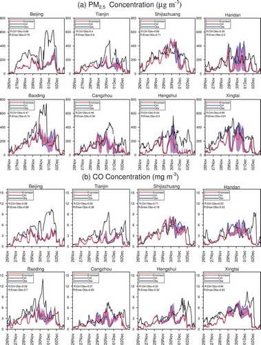
To illustrate the model performance regarding PM_2.5 simulation, the hourly evolution of PM_2.5 concentration at the eight cities during 26 November to 2 December from both observation and CTRL model output are shown in Figure 2(a). Intuitively, the hourly PM_2.5 concentration fluctuated intensively, with sharp increases in BJ, BD, and HS especially. These anomalous fluctuations may have been caused by the rapid movement of locally contaminated air masses, which may have derived from the boundary layer jet or local valley wind circulation (Liao et al. 2016; Chen et al. 2018). However, the CTRL run of the WRF-Chem model showed quite different performance regarding PM_2.5 in the eight cities. The R varied between 0.29 and 0.69 (above 0.6 at BJ, SJZ and XT; between 0.4 and 0.5 at TJ, BD, CZ and HS). Specifically, the simulation underestimated the concentration during peak-sustaining stage (roughly 29 November to 1 December) at BJ, TJ, BD, CZ, and HS. The abovementioned sharp increases of PM_2.5 concentration were all missed by CTRL. Therefore, it is a challenge for WRF-Chem to simulate such a long-lasting (7 days) extreme haze pollution event — especially the sudden increase or decrease of instantaneous PM_2.5 concentration.

Figure 2. (a) Hourly PM_2.5 concentration time series in eight cities predicted by CTRL (blue line), the INBDDE ensemble mean (red line), and the observation (black line). Pink filling represents the maximum and minimum range (or dispersion) of the forecasting results of 10 ensemble members. The correlation coefficients between the forecasting concentration of CTRL, INBDDE and the observed values are marked on the left-hand side. The bottom panel (b) is the same as (a), but for CO.

3.2 Ensemble simulation results

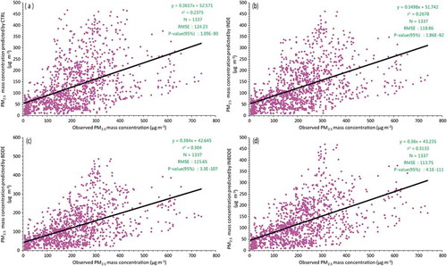
In order to evaluate the forecasting skills of the three groups of ensemble experiments (i.e., INDE, BDDE, INBDDE), a series of linear fitting and regression analyses were performed for the hourly PM_2.5 concentration between observation and CTRL, the ensemble mean values of ensemble runs. There are a total of 1337 valid sample points (7 (days) × 24 (hours) × 8 (cities), removing 7 missing values) in the four scatterplots shown in Figure 3. The r² statistic — usually referred to as the determination coefficient, the ratio of regression variance to observation variance — is a statistical measure of how close the data are to the fitted regression line (Huang 2004).

Figure 3. Scatterplots of the observed PM_2.5 concentration (units: μg m⁻³) in eight cities and the predicted PM_2.5 concentration from (a) CTRL, (b) INDE, (c) BDDE and (d) INBDDE, respectively. The black lines indicate the linear trend estimation based on the least-squares method.

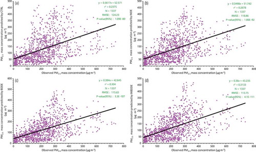
In contrast to the single, deterministic initial conditions and LBCs in CTRL, all of the three groups of ensemble runs did indeed improve the prediction skill of PM_2.5 concentration. The r² (RMSE) increased (decreased) from 0.24 (124.23) in CTRL to 0.31 (113.75) in INBDDE (cf. Figure 3(a,d). Not limited to PM_2.5, INBDDE showed the best performance in terms of the surface meteorological variables, followed by BDDE and INDE (Table 2). The ensemble simulation experiment that simultaneously changed the initial conditions and LBCs (i.e., INBDDE) was an effective method to improve PM_2.5 forecasting compared to only changing the initial conditions (INDE) or LBCs (BDDE), in this case. However, what was modulating the variation in PM_2.5 concentration in the INBDDE experiment? We further examined the variation of near-surface meteorological factors to understand the possible mechanism.

Table 2. Statistics of PM_2.5 concentration (units: μg m⁻³) and surface meteorological variables in CTRL, INDE, BDDE, and INBDDE. RH2M and T2M denote the relative humidity (units: %) and temperature (units: °C) at 2 m near the ground; WS10 and WD10 denote the wind speed (units: m s⁻¹) and direction (units: °) at 10 m near the ground. The ensemble mean values of the above variables were used to compute the statistical parameters in INDE, BDDE, and INBDDE.

Variable	Number of samples	Experiment	Bias	R	RMSE	EE
PM2.5 (μg m^−3)	1337	CTRL	−77.95	0.49	124.23	0
		INDE	−81.20	0.52	118.86	−4.33%
		BDDE	−83.32	0.55	115.65	−6.91%
		INBDDE	−87.63	0.56	113.75	−8.44%
RH2M (%)	1337	CTRL	−7.24	0.78	13.38	0
		INDE	−7.84	0.79	13.23	−1.10%
		BDDE	−6.85	0.78	13.47	0.70%
		INBDDE	−7.48	0.79	13.49	0.81%
T2M (°C)	1336	CTRL	0.26	0.83	2.04	0
		INDE	0.41	0.83	2.01	−1.20%
		BDDE	0.24	0.83	2.04	0.13%
		INBDDE	0.37	0.83	2.04	0.03%
WS10(m s^−1)	1336	CTRL	1.31	0.61	1.47	0
		INDE	1.32	0.62	1.46	−0.75%
		BDDE	1.29	0.64	1.48	0.56%
		INBDDE	1.30	0.64	1.50	2.32%
WD10 (°)	1336	CTRL	−16.84	0.26	133.29	0
		INDE	−18.89	0.27	126.37	−5.19%
		BDDE	−14.74	0.29	121.45	−8.89%
		INBDDE	−15.73	0.29	120.49	−9.61%

Table 2 gives the model bias, R, RMSE, and EE of the four groups of experiments. For PM_2.5 concentration, the RMSE (R) decreased (increased) from 124.23 (0.49) in CTRL to 118.86 (0.52) in INDE, 115.65 (0.55) in BDDE, and 113.75 (0.56) in INBDDE. As for all the other variables, WRF-Chem showed consistent biases in each experiment group. The EE was −4.33%, −6.91%, and −8.44% in INDE, BDDE, and INBDDE, respectively. The slight variations of R and RMSE in 2-m relative humidity and temperature among all the ensemble experiments indicated that the variations of initial conditions and LBCs had little effect on the simulations of these two variables. Despite the weak increase in the RMSE of wind speed in INBDDE, the decrease in the RMSE of wind direction in three ensemble groups (−5.19%, −8.89%, and −9.61%) seemed to be more dominant. Because we performed an eight-day simulation, the simulation of wind direction was more sensitive to the ensembles of the LBCs than those of the initial conditions in this case study. Also, the ensemble scheme involving simultaneously changing the initial conditions and LBCs led to the best performance for both wind direction and PM_2.5 concentration. Wind direction variation means that the regional transportation of PM_2.5 among cities may be changed, despite wind speed remaining steady. Next, we discuss the changes in PM_2.5 spatial distribution caused by the wind direction adjustment in INBDDE (with the most obvious variations).

Figure 2 shows the hourly evolution of PM_2.5 and CO concentration in the eight cities from observations, CTRL and INBDDE ensemble means. In contrast to CTRL, the PM_2.5 concentration in INBDDE decreased in southern cities of the megacity cluster (HD, HS, and XT), but increased in northern cities (BJ, TJ, BD, and CZ), roughly from 28 November to 1 December. The dispersion among ensemble members in INBDDE tended to decrease in southern cities. The R of PM_2.5 in XT, HD, and HS (southern cities) decreased from 0.69, 0.29 and 0.42 in CTRL to 0.61, 0.2, and 0.3 in INBDDE. But, the R in BJ, TJ, BD, and CZ (northern cities) increased from 0.66, 0.4, 0.47 and 0.48 in CTRL to 0.75, 0.6, 0.74 and 0.56. Based on these analyses, it can be roughly concluded that the INBDDE ensemble mean improved the prediction skill of the regional transport of atmospheric pollutants, i.e., PM_2.5 from the southern cities to the northern cities, which will reduce the pollution in the southern region but aggravate it in the northern region, and finally lead to an overall good simulation.

CO is a kind of inactive gas, which is a good indicator for analysis of air pollutant transportation. It is difficult for CO to participate in atmospheric chemical reactions near 0°C, which means the observed CO concentration is mainly affected by the co-effects of local source emissions and cross-regional transmission (Saide et al. 2011). So, we used CO as a tracer gas to test the hypothesis. In Figure 2(b), CO shows a similar evolution trend with PM_2.5 in the eight cities from 29 November to 1 December: the CO concentrations in the INBDDE ensemble mean are lower in HD, HS, and XT than those in CTRL, but higher in TJ, BD, and CZ. Therefore, it is possible that INBDDE performs better in capturing the effect of intraregional transmission or variation of near-surface wind direction on PM_2.5 than the CTRL simulation.

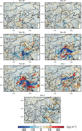
We used the spatial difference fields to further understand the above transportation processes (Figure 4). On 26 and 27 November, there was no significant redistribution of PM_2.5, with fewer surface wind differences. From 28 November, the southerly wind anomaly appeared in the south-to-central part of Hebei Province. The southerly wind anomaly strengthened on 29 November and reached its peak of over 1 m s⁻¹ on 30 November. Due to the sustained anomalous southerly wind, the PM_2.5 concentration in southern Hebei began to reduce on 28 November, and then this phenomena further extended to central Hebei on 29 November. In contrast, the PM_2.5 concentration increased distinctly in central to northern Hebei on the same day. On 30 November, the PM_2.5 concentration in southern Hebei reduced by more than 80 μg m⁻³, while it increased by more than 60 μg m⁻³ in central to northern Hebei, which corresponded to 27% and 32% of the daily mean PM_2.5 concentration predicted by CTRL in HD and BD (288.5 μg m⁻³ and 185.9 μg m⁻³), respectively. The differences weakened on 1 December and tended to disappear on 2 December. Therefore, in the INBDDE ensemble runs, the pollutants located in southern Hebei Province were transported to the northern region through locally strengthened southerly wind. This redistribution of the PM_2.5 concentration resulted in the overall improvement in the eight cities.

Figure 4. Differences of daily mean PM_2.5 concentration (shaded; units: μg m⁻³) and 10 m wind vector between the INBDDE ensemble mean and CTRL from 26 November to 2 December.

4. Summary and conclusion

In this paper, we investigated the sensitivity of PM_2.5 concentration evolution to meteorological field variations through a series of numerical experiments with the WRF-Chem model. A seven-day, long-lasting extreme haze pollution event over the BTH megacity cluster was selected. Based on ERA5 reanalysis data and 10 EDA members, we carried out a CTRL and three groups of ensemble experiments with different meteorological initial conditions and LBCs. The CTRL run reproduced well the meteorological conditions and the overall life cycle of the haze event over the BTH region. However, it failed to capture the sudden increase or decrease in instantaneous PM_2.5 concentration in the eight selected cities. In general, the ensemble experiments improved the simulation – especially that of PM_2.5 concentration. Compared with CTRL, the RMSE of PM_2.5 concentration decreased by 4.33%, 6.91%, and 8.44% in INDE, BDDE, and INBDDE, respectively. This implies that the PM_2.5 concentration predicted by WRF-Chem is sensitive to the background meteorological field.

In fact, there was little improvement in the near-surface meteorological variables (e.g., 2-m relative humidity, temperature and 10 m wind speed) in the three groups of ensemble experiments, except the 10 m wind direction. It was found that the RMSE decreases of 10-m wind direction (−5.19%, −8.89%, and −9.61%) seemed to be the dominant reason for the improvement in PM_2.5 prediction skill in the three groups of ensemble experiments. For example, in the INBDDE run, the initial conditions and LBC ensemble schemes resulted in an increased southerly wind anomaly (compared to CTRL) in the southern part of Hebei Province, which consequently led to northward transport of PM_2.5 and therefore improved the PM_2.5 concentration spatial distribution — especially in the northern part of the BTH region. In conclusion, based on this case, the initial conditions and LBCs–based ensemble scheme is an effective method to improve the prediction skills of wind direction and PM_2.5 concentration by using the WRF-Chem model.

It should be mentioned that a sharp increase or decrease in PM_2.5 concentration has happened frequently in recent years, which presents a great challenge for both real-time air quality prediction and numerical simulation studies. The ensemble schemes in this paper are expected to provide a possible way for air quality forecasting. Also, it may be a potential way to make ensemble forecasts by simultaneously considering both meteorological conditions and physical/chemical parameterization schemes to reduce the random errors.

Acknowledgments

The ERA5 data used in this study are available from https://www.ecmwf.int/en/forecasts/datasets/reanalysis-datasets

Disclosure statement

No potential conflict of interest was reported by the authors.

Supplementary material

Supplemental data for this article can be accessed here

Additional information

Funding

This work was jointly supported by the National Basic Research (973) Program of China [grant number 2015CB954102], the National Natural Science Foundation of China [grant number 41475043], and the National Key R&D Program of China [grant number 2018YFC1507403].

References

- Cai, W., K. Li, H. Liao, H. Wang, and L. Wu. 2017a. “Weather Conditions Conducive to Beijing Severe Haze More Frequent under Climate Change.” Nature Climate Change 7: 257–262. doi:10.1038/NCLIMATE3249.
- Cai, Z., Y., . Q. Yao, S. Q. Han, T. Y. Hao, and J. L. Liu. 2017b. “Ensemble Forecast Experiments of PM2.5 Based on Multiple Boundary Layer Schemes in Tianjin.” (in Chinese). Journal of Applied Meteorological Science 5: 611–620.
- Chapman, E. G., W. I. Gustafson Jr, R. C. Easter, J. C. Barnard, S. J. Ghan, M S. Pekour, and J D. Fast. 2009. “Coupling Aerosol-cloud-Radiative Processes in the WRF-Chem Model: Investigating the Radiative Impact of Elevated Point Sources.” Atmospheric Chemistry and Physics 9 :945–964. doi:10.5194/acp-9-945-2009.
- Chen, Y., J. L. An, Y. L. Sun, X. Q. Wang, Y. Qu, J. Zhang, Z. Wang, and J. Duan. 2018. “Nocturnal Low-level Winds and Their Impacts on Particulate Matter over the Beijing Area.” Advances in Atmospheric Sciences 35 (12): 1455–1468. doi:10.1007/s00376-018-8022-9.
- Cheng, X. H., X. D. Xu, X. Q. An, Y. C. Jiang, Z. Y. Cai, Z. G. Diao, and D. P. Li. 2016. “Inverse Modeling of SO2 and NOx Emissions Using an Adaptive Nudging Scheme Implemented in CMAQ Model in North China during Heavy Haze Episodes in January 2013.” (in Chinese). Acta Scientiae Circumstantiae 36: 638–648.
- Crippa, P., R. C. Sullivan, A. Thota, and S. C. Pryor. 2019. “Sensitivity of Simulated Aerosol Properties over Eastern North America to WRF-Chem Parameterizations.” Journal of Geophysical Research. doi:10.1029/2018JD029900.
- Grell, G. A., S. E. Peckham, R. Schmitz, S. A. McKeen, G. J. Frost, et al. 2005. “Fully Coupled ‘online’ Chemistry in the WRF Model.” Atmospheric Environment 39 (37): 6957–6976. doi:10.1016/j.atmosenv.2005.04.027.
- He, Y. J. 2018. “A DRP-4DVar-based Coupled Data Assimilation Method and Its Application in Decadal Predictions” (in Chinese). Doctoral dissertation, Tsinghua University, 119pp.
- Huang, J. Y. 2004. Methods of Meteorological Statistical Analysis and Forecasting. (in Chinese).Beijing: China Meteorological Press. 298.
- Huang, S., X. Tang, W. S. Xu, Z. Wang, H. S. Chen, J. Li, Q. Z. Wu, and Z. F. Wang. 2015. “Application of Ensemble Forecast and Linear Regression Method in Improving PM10 Forecast over Beijing Areas.” (in Chinese). Acta Scientiae Circumstantiae 35 (1): 56–64. doi:10.13671/j.hjkxxb.2014.0728.
- Ji, D. S., L. Li, Y. S. Wang, J. K. Zhang, M. T. Chen, Y. Sun, Z. Liu, et al.2014. “The Heaviest Particulate Air-pollution Episodes Occurred in Northern China in January, 2013: Insights Gained from Observation.” Atmospheric Environment 92 :546–556. doi:10.1016/j.atmosenv.2014.04.048.
- Li, J., H. Y. Du, Z. F. Wang, Y. L. Sun, W. Y. Yang, J. Li, X. Tang, and P. Fu. 2017. “Rapid Formation of a Severe Regional Winter Haze Episode over a Mega-city Cluster on the North China Plain.” Environmental Pollution 223 :605–615. doi:10.1016/j.envpol.2017.01.063.
- Li, K., H. Liao, W. J. Cai, and Y. Yang. 2018. “Attribution of Anthropogenic Influence on Atmospheric Patterns Conducive to Recent Most Severe Haze over Eastern China.” Geophysical Research Letter 45: 2072–2081. doi:10.1002/2017GL076570.
- Li, M., Q. Zhang, D. G. Streets, K. B. He, Y. F. Cheng, L K. Emmons, H. Huo, et al. 2014. “Mapping Asian Anthropogenic Emissions of Non-methane Volatile Organic Compounds to Multiple Chemical Mechanisms.” Atmospheric Chemistry and Physics 14 :5617–5638. doi:10.5194/acp-14-5617-2014.
- Liao, X. N., Z. B. Sun, N. He, P. S. Zhao, and Z. Q. Ma. 2016. “A Case Study on the Rapid Cleaned Away of PM2.5 Pollution in Beijing Related with BL Jet and Its Mechanism.” Environmental Science (in Chinese) 37 (1): 51–59. doi:10.13227/j.hjkx.2016.01.008.
- Liu, F., Q. Zhang, D. Tong, B. Zheng, M. Li, H. Huo, and K. B. He. 2015. “High-resolution Inventory of Technologies, Activities, and Emissions of Coal-fired Power Plants in China from 1990 to 2010.” Atmospheric Chemistry and Physics 15 :13299–13317. doi:10.5194/acp-15-13299-2015.
- Mallet, V., G. Stoltz, and B. Mauricette. 2009. “Ozone Ensemble Forecast with Machine Learning Algorithms.” Journal of Geophysical Research Atmospheres 114: D053307. doi:10.1029/2008JD009978.
- Peckham, S., G. A. Grell, S. A. McKeen, M. Barth, G. Pfister, C. Wiedinmyer, J. D. Fast, et al. 2011. “WRF-Chem Version 3.3 User’s Guide.” NOAA Technical Memo, 98.
- Petersen, A. K., G. P. Brasseur, I. Bouarar, J. Flemming, M. Gauss, F. Jiang, and R. Kouznetsov. 2018. “Ensemble Forecasts of Air Quality in Eastern China – Part 2. Evaluation of the MarcoPolo-Panda Prediction System, Version 1.” Geoscientific Model Development Discussions. doi:10.5194/gmd-2018-234.
- Powers, J. G., J. B. Klemp, W. C. Skamarock, C. A. Davis, J. Dudhia, D. O. Gill, J. L. Coen, and D. J. Gochis. 2016. “The Weather Research and Forecasting Model: Overview, System Efforts, and Future Directions.” AMS. doi:10.1175/BAMS-D-15-00308.1.
- Quan, J. N., X. X. Tie, Q. Zhang, Q. Liu, X. Li, Y. Gao, and D. Zhao. 2014. “Characteristics of Heavy Aerosol Pollution during the 2012–2013 Winter in Beijing, China.” Atmospheric Environment 88 :83–89. doi:10.1016/j.atmosenv.2014.01.058.
- Saide, P. E., G. R. Carmichael, S. N. Spak, L. Gallardo, A. E. Osses, M A. Mena-Carrasco, and M. Pagowski. 2011. “Forecasting Urban PM10 and PM2.5 Pollution Episodes in Very Stable Nocturnal Conditions and Complex Terrain Using WRF–Chem CO Tracer Model.” Atmospheric Environment 45 (16): 2769–2780. doi:10.1016/j.atmosenv.2011.02.001.
- Skamarock, W. C., J. B. Klemp, J. Dudhia, D. O. Gill, D. M. Barker, W. Wang, and J. G. Powers. 2008. “A Description of the Advanced Research WRF Version 3.” NCAR Tech Note NCAR/TN-475+STR: 113. doi:10.5065/D68S4MVH.
- Sun, Y. L., Z. F. Wang, O. Wild, W. Q. Xu, C. Chen, W. Du, L. Zhou, Qi Zhang, T. Han, Q. Wang, X. Pan, H. Zheng, J. Li, X. Guo, J. Liu, D R. Worsnopet al. 2016. ““APEC Blue”: Secondary Aerosol Reductions from Emission Controls in Beijing.” Scientific Reports 6 :20668. doi:10.1038/srep20668.
- Tang, X., Z. F. Wang, J. Zhu, A. Gbaguidi, and Q. Z. Wu. 2010. “Ensemble-Based Surface O3 Forecast over Beijing.” Climatic and Environmental Research (in Chinese) 15 (5): 677–684. doi:10.3878/j.issn.1006-9585.2010.05.18.
- Tuccella, P., G. Curci, C. Visconti, B. Bessagnet, L. Menut, and R J. Park. 2012. “Modeling of Gas and Aerosol with WRF/Chem over Europe: Evaluation and Sensitivity Study.” Journal of Geophysical Research 117 :D03303. doi:10.1029/2011JD016302.
- Wang, L. Q., P. F. Li, S. C. Yu, K. Mahmood, Z. Li, S. Chang, W. Liu, D. Rosenfeld, R C. Flagan, and J H. Seinfeld. 2018. “Predicted Impact of Thermal Power Generation Emission Control Measures in the Beijing-Tianjin-Hebei Region on Air Pollution over Beijing, China.” Scientific Reports 8 (1): 934. doi:10.1038/s41598-018-19481-0.
- Wang, Z. F., Q. Z. Wu, A. Gbaguidi, P. Z. Yan, W. Zhang, W. Wei, and X. Tang. ; 2009. “Ensemble Air Quality Multi-Model Forecast System for Beijing (ems-beijing): Model Description and Preliminary Application.” (in Chinese) Journal of Nanjing University of Information Science & Technology 2009 (1): 19–26.
- Wu, P., Y. H. Ding, and Y. J. Liu. 2017. “Atmospheric Circulation and Dynamic Mechanism for Persistent Haze Events in the Beijing–Tianjin–Hebei Region.” Advances in Atmospheric Sciences 34 (4): 429–440. doi:10.1007/s00376-016-6158-z.
- Xu, P., Y. F. Chen, and X. J. Ye. 2014. “Haze, Air Pollution, and Health in China.” The Lancet 382 (9910): 2067. doi:10.1016/S0140-6736(13)62693-8.
- Yang, Y. R., X. G. Liu, Y. Qu, J. L. Wang, J. L. An, Y. Zhang, and F. Zhang. 2015. “Formation Mechanism of Continuous Extreme Haze Episodes in the Megacity Beijing, China, in January 2013.” Atmospheric Research 155 :192–203. doi:10.1016/j.atmosres.2014.11.023.
- Žabkar, R., D. Koračin, and J. Rakovec. 2013. “A WRF/Chem Sensitivity Study Using Ensemble Modelling for A High Ozone Episode in Slovenia and the Northern Adriatic Area.” Atmospheric Environment 77: 990–1004. doi:10.1016/j.atmosenv.2013.05.065.
- Zhang, Y., M. Bocquet, V. Mallet, C. Seigneur, and A. Baklanov. 2012. “Real-time Air Quality Forecasting, Part I: History, Techniques, and Current Status.” Atmospheric Environment 60 :632–655. doi:10.1016/j.atmosenv.2012.06.031.
- Zhang, Z. Y., D. Y. Gong, S. J. Kim, R. Mao, J. Xu, X. Zhao, and Z. Ma. 2017. “Cause and Predictability for the Severe Haze Pollutions in Downtown Beijing during November–December 2015.” Science of the Total Environment 592 :627–638. doi:10.1016/j.scitotenv.2017.03.009.
- Zheng, Z. 2013. “Statistical Analysis of the Effects of Urbanization on Haze Days in Beijing Area.” (in Chinese). Ecology and Environmental Sciences 22(8): 1381–1385.