Overview of the 9th Chinese National Arctic Research Expedition

ABSTRACT

The 9th Chinese National Arctic Research Expedition was carried out from 20 July to 26 September 2018. The expedition was successful in undertaking multidisciplinary comprehensive surveys in the fields of physical oceanography, marine meteorology, sea ice, marine chemistry, marine biology, marine ecology, geology, and geophysics in the Bering Sea, Chukchi Sea, Chukchi Plateau, Mendeleev Ridge, and Canada Basin. This paper gives an overview of the main achievements of this expedition and highlights the scientific achievements.

Graphical Abstract

摘要

中国第9次北极考察航次于2018年7月20日至9月26日执行，在白令海、楚科奇海、楚科奇海台、门捷列夫海岭和加拿大海盆开展了物理海洋、海洋气象、海冰、海洋化学、海洋生物、海洋生态、地质和地球物理等多学科综合考察。本文对中国第9次北极考察取得的主要成果进行了概述。

KEYWORDS:

• Chinese National Arctic Research Expedition
• Chukchi Sea
• Canada Basin
• Bering Sea
• Arctic Ocean

关键词:

• 中国第9次北极考察；楚科奇海；加拿大海盆；白令海；北冰洋

1. Introduction

Because of the Arctic amplification of climate warming, the extent and thickness of Arctic sea ice have declined dramatically in recent decades (Parkinson and Comiso 2013; Lindsay and Schweiger 2015), which dominates the sea-ice loss at the global scale (Simmonds 2015). The loss of Arctic sea ice extent has been most remarkable in summer, with the Arctic-wide melt season having been lengthened at a rate of 5 d/10 yr during 1979–2013 (Stroeve et al. 2014). Regionally, the most obvious retreat of Arctic sea ice has occurred in the Pacific sector during the summer (Xia, Xie, and Ke 2014; Lei et al. 2017).

The 9th Chinese National Arctic Research Expedition (CHINARE) was the first Arctic expedition since the Chinese government published its white paper entitled ‘China’s Arctic Policy’. The 9th CHINARE focused on the change in Arctic sea ice and its response to climate change, its influences on the environment and ecosystem in the Arctic region, as well as the main behaviours of ocean–ice–atmosphere interaction at multiple scales.

The 9th CHINARE began on 20 July 2018 and it ended on 26 September 2018. The research vessel (R/V), Xuelong, reached its most northerly location of 84°48ʹN on 20 August 2018. The expedition guaranteed the implementation of 13 operational projects, 9 national scientific research projects, and 3 international cooperation projects. Two foreign scientists from France and one from the United States attended this expedition.

The expedition was successful in undertaking multidisciplinary comprehensive surveys in the fields of physical oceanography, marine meteorology, sea ice, marine chemistry, marine biology, marine ecology, geology, and geophysics in areas of the Bering Sea, Chukchi Sea, Chukchi Plateau, Mendeleev Ridge, and Canada Basin.

2. Main achievements

2.1. Physical oceanography and marine meteorology

The main tasks of the physical oceanographic and marine meteorological surveys included transect investigations, glider observations, and surface temperature, salinity, and meteorological observations during navigation.

2.1.1. Transect hydrographic investigations

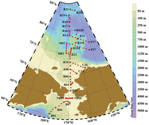
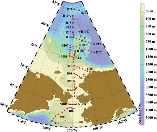
Hydrographic investigations were conducted using conductivity–temperature–depth (CTD) and lowered acoustic Doppler current profiler (LADCP) sensors in the Pacific section of the Arctic Ocean. Overall, CTD/LADCP operations were performed at 88 stations during the expedition (Figure 1). Compared with historical voyage data collected during the previous CHINARE cruises from 1999 to 2012, the temperature and salinity south of the Bering Strait were slightly higher in 2018. Historical records showed a cold-water mass in the Bering Strait characterized by water temperatures of < 2°C. In-situ data from the 9th CHINARE revealed that the temperature of the water mass was > 3°C. The water mass characterized by salinity of < 32 was also markedly reduced in 2018. The physical mechanism for such moderate abnormalities of water mass is worthy of further study.

Figure 1. Locations of oceanographic investigation stations.

2.1.2. Glider observations

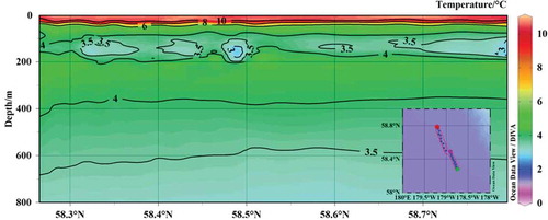
This expedition successfully conducted continuous high-frequency glider (‘Haiyi’, built at the Shenyang Institute of Automation, Chinese Academy of Sciences) observations in the basin and continental slope region of the Bering Sea. It marked the first deployment of a glider to perform hydrographic investigations in this region during CHINARE cruises. The glider operated for 45 days, and during this period it sailed nearly 930 km and obtained 229 profiles of temperature and salinity. The temperature profiles revealed a water mass with temperatures of < 4°C centred at the depth of 170 m over the continental slope of the Bering Sea (Figure 2). The lowest temperature of this water mass was < 3°C, with a depth of approximately 100 m. As the properties of this water mass were the same as the surface water in winter and the mixing depth of the upper layer in summer was no more than 100 m, this water mass was identified as residual surface water in winter. The successful launch and operation of the glider in this boreal region proved that underwater vehicles are a useful supplement to ship-based oceanographic surveys.

Figure 2. Temperature distribution obtained by the glider in the Bering Sea.

2.1.3. Sea surface temperature and salinity observations during sailing

Observations of sea surface temperature and salinity were performed throughout the expedition except for a temporary suspension at high latitudes where the sampling system became frozen. Overall, both sea surface temperature and salinity generally decreased from south to north. The sea surface temperature was above 0°C in the southern waters of the Bering Sea and the Chukchi Sea, and around −1.5°C in the region north of 73°N, which indicated that the sea ice in this region was in the melting stage. Salinity was found to be > 31 in the region south of the Bering Strait, with little variation, whereas it decreased to 30 in the region north of 73°N, which highlighted the contribution of meltwater of sea ice to the freshening of the ocean mixing layer.

2.1.4. Marine meteorological observations during sailing

Marine meteorological observations, including cloud amount, cloud type, weather phenomena, swell waves, and sea ice were performed during the expedition. The cruise experienced some extreme synoptic events such as extratropical cyclones and polar lows, which intruded into the Arctic Ocean. Cyclones can bring more warm and moist air masses from the low latitudes, especially from the Nordic Sea, which would affect the moisture and radiation balance over the ice surface. Nevertheless, the expedition encountered the storms with wind intensities reaching above level 6 on 13 occasions. During the expedition, the wind direction was primarily southwesterly, westerly, and southerly.

2.1.5. GPS sounding observations

In the region north of 55°N, sounding balloons were launched two to three times each day at 0000, 0600, and 1200 UTC, as a contribution to the Year of Polar Prediction (YOPP). The height of the lapse rate tropopause (LRT) was 7.45–11.13 km, with an average height of 9.42 km. The temperature of the LRT in different regions was between −60.0°C and −40.1°C, with an average temperature of −51.8°C.

2.2. Sea-ice observations

2.2.1. Sea-ice concentration and thickness observations during sailing in the ice region

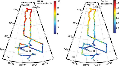
Sea-ice concentration and thickness observations were conducted at the long-term and short-term ice stations during the expedition (Figure 3). An ice edge appeared at about 73°N and the sea ice thickness gradually increased from 73°N to reach a maximum of approximately 2.0 m for level ice at around 84°N (Figure 4). The concentration of sea ice increased considerably in the area north of 82°N, where the ice concentration was found close to 95% and could be identified as a pack-ice zone. Along the southward leg of the expedition after 28 August 2018, the thickness of sea ice in the region south of 82°N decreased markedly, where the ice was still in the melt stage during this period. On 30 August 2018, the half-hour average of sea-ice thickness in the marginal sea-ice zone was < 0.7 m. The melting process of sea ice was related to both thermodynamic and dynamic processes of ice.

Figure 3. Locations of ship-based and ice-based sea-ice observations. Also shown are the serial numbers of the short-term stations according to their implementation time.

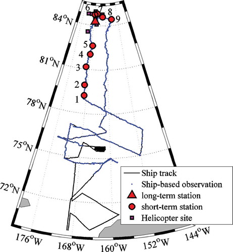
Figure 4. Spatial distribution of sea-ice (a) concentration and (b) thickness.

2.2.2. Physical structure of the snow and ice

During the 9th CHINARE, several short-term ice stations were set up to collect samples for the determination of the texture and physical structure of the snow and ice. Thus, snow density and water content within the snow cover were obtained from 45 sets of snow profiles. We collected 54 sea-ice cores and obtained their temperature, salinity, density, texture, structure, and mechanical properties. The snow depth was 0.07–0.12 m, with an average of 0.09 m, and most comprised coarse-grained snow. The average water content and density of the sampled snow were 0.75% and 0.24 g cm⁻³, respectively. The second and fifth short-term ice stations featured thick and multi-year ice. The minimum ice thickness was 0.93 m and the maximum ice thickness was 5.77 m. Short-term ice stations were mostly selected at the floes with obvious ice ridges. Therefore, the average ice thickness was 2.01 m. The average salinity of sea ice was between 1.23 PSU and 2.92 PSU. The lowest salinity, at the sixth short-term ice station, was 1.23 PSU, and the highest salinity, at the first short-term ice station, was 2.92 PSU. From the ice-core measurements it was found that the salinity of the ice surface was close to 0 PSU. The main reason was that the salinity of sea ice is determined by the content of brine in the ice layer. In summer, the temperature is higher, the surface sea ice melts substantially, and the large amount of brine discharged leads to the interconnection of brine channels. The brine content in the ice decreased significantly, making the salinity close to 0 PSU. Sea-ice density ranged from 500 to 950 kg m⁻³, and the average density of each ice station ranged from 832 to 871 kg m⁻³. The highest average density, observed at the first short-term ice station, was 871 kg m⁻³, and the lowest, observed at the ninth short-term ice station, was 832 kg m⁻³. From the ice-core measurements, it was found that the density of sea ice was relatively low. The average density of sea ice in the top 0–0.10 m layer of each ice station was 662 kg m⁻³, which was significantly lower than the average density of sea ice measured in this time. The main reason was that the surface snow will melt and freeze to form snow ice, and the structure was also loose.

2.2.3. Sea-ice drift and mass balance observations

Sea-ice drift was obtained using the GPS data measured by the ice-tethered buoys and the sea-ice mass balance was measured by an unmanned ice station built at the Polar Research Institute of China. The drift trajectories of the buoys showed that the sea ice initially moved eastwards, but then moved towards the southeast from 28 August 2018 onwards at a speed of 0.01–0.35 m s⁻¹. The sea-ice trajectory might have been responding to cyclone activity. The data measured by the unmanned ice station showed that the ice thickness decreased from 1.42 to 1.32 m from 18 August to 1 September. The melting rate of 0.0067 m d⁻¹ was equivalent to a latent heat flux of 20 W m⁻². The deployment of the unmanned ice station allowed us to observe the thermodynamic processes of sea ice from summer to winter.

2.2.4. Sea-ice optical properties observation

We conducted observations of the optical properties of Arctic melt ponds at seven ice stations. The results showed that frozen melt ponds have the highest albedo in the 490-nm band, reaching 0.35. The albedo above the 700-nm band is relatively small, with a value of about 0.1. With a decrease of solar inclination angle, the spectrum with higher albedo (e.g., the 500-nm band) was found to increase slightly, while the albedo of the 700-nm band remained stable. The observed reflection of irradiance of melt ponds was found to exhibit diurnal changes. Observations of snow albedo were conducted at six ice stations. The albedo spectra at some short-term ice stations (18ICE02–18ICE04) were found to be similar, with an integrated albedo of 0.56–0.71 at 300–920 nm; however, the albedo spectra at other short-term ice stations (18ICE06, 18ICE08, and 18ICE09) were different. At ice station 18ICE06, the reflection in the 300–500-nm band was found to be markedly enhanced, with an integrated albedo of 0.95. Integrated albedos of 0.63 and 0.67 were observed at short-term ice stations 18ICE08 and 18ICE09, respectively. The main reason for this phenomenon is that old snow with large granules had been covered by some fresh snow.

2.3. Marine geological observations

2.3.1. Characteristics of seafloor sediment

The characteristics of sediments vary obviously in different regions. The study region can be divided into four sedimentary areas based on sediment composition, grain size, color, and odor of the obtained sediment sample. In the Chukchi Plateau area, the sediment is characterized by its brown color and uneven thickness, and it comprises mostly silty clay. On the continental slope of the Chukchi Sea, the seafloor sediment is gray-green clay silt or sandy silt. Below that, the seafloor sediment is dark gray or black clay silt rich in organic matter and it has an odor of hydrogen sulfide. In the Bering Strait and the northern Bering Sea, the seafloor comprises bedrock or gravel sediment. The sedimentary features of the Bering Sea shelf are similar to those of the Chukchi Sea shelf.

2.3.2. Polymetallic nodules

The 9th CHINARE conducted seabed rock dredges and benthos trawling on the Chukchi Plateau. Along the BT transect, a large number of iron-manganese nodules/crusts were found by rock dredges (1 station) and benthos trawling (10 stations). This represented the second time that the presence of iron-manganese nodules/crusts had been detected in the CHINARE cruises following the discovery of nodules/crusts through benthos trawling near the Chukchi Plateau during the 7th Chinese Arctic Research Expedition. The polymetallic nodules found in this expedition were in a region located to the south of the U.S. investigation area. The water depth of the stations was < 350 m, except at station DR2 (water depth > 1000 m). Most of the polymetallic nodules were 1–2-cm thick with a platy structure; however, some had a nodule-like crust and a crusty structure. The formation of polymetallic nodules/crusts is symbiotic with the seafloor sediments. The morphology and thickness of the polymetallic nodules/crusts were found comparable with those reported by the United States (Hein et al. 2017) and from the Russian Mendeleev Ridge (Konstantinova et al. 2017).

2.4. Marine geophysical investigation

2.4.1. Submarine topographic survey

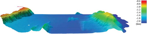
A multibeam survey was conducted at the edge of the Chukchi Sea and along a transect in the Canada Basin. The main survey lines were distributed in the areas of the Chukchi Platform, Chukchi Abyssal plain, Northwind Ridge, and Canada Basin. The measured bathymetric data showed various types of morphology, including glacial landforms, seabed valleys, the abyssal plain, and seamounts. We conducted a full-covered high-resolution multibeam survey in the Northwind basin (Figure 5). On the Northwind Ridge, the topography is rather flat with a water depth between 1950 and 2050 m. Inside the Northwind basin, the prominent topographic features are the volcanic ridges and seamounts.

Figure 5. Volcanic ridges and seamounts in the Northwind basin.

2.4.2. Rock dredges

Based on the topography determined by the multichannel survey, we selected two stations in the steepest area in the Chukchi Borderland to perform rock dredges. According to the roundness of the sample and the cable tension, the collected samples were primarily divided into ice-rafted debris and in-situ outcrops. The in-situ rocks contained amphiboles and feldspars, which is similar to the basement rock of the Canadian Arctic Archipelago, suggesting that the two regions might have been conjugative prior to the opening of the Amerasian Basin.

2.5. Marine chemistry observations

2.5.1. Nutrient distribution

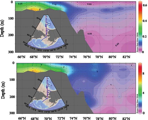
The distributions of nitrite and ammonia with latitude and water depth along the R section are shown in Figure 6. The average nitrite concentration on the shelf (water depth < 100 m) reached 0.25 µM, compared to 0.06 µM of the average content in the basin (water depth > 100 m). Meanwhile, the average concentration of ammonia on the shelf was 3.87 µM, and the concentration of ammonia in the deep basin was quite low. Nutrient distributions showed obvious change in both the horizontal and vertical directions. In the horizontal direction, the nutrient content on the shelf was significantly higher than that in the deep basin. In the vertical direction, the distribution pattern of nutrients in the shelf area and deep basin was also different, with nitrite and ammonia increased with water depth on the shelf and having subsurface maxima in the deep basin.

Figure 6. Distribution of nitrite and ammonia (µM) along the R transect in the western Arctic Ocean.

2.5.2. Ocean acidification observations

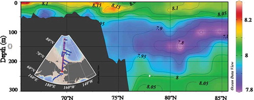
The distribution of pH (total scale, at in-situ temperature) along the R transect is stratified from bottom to surface in Figure 7. Also, the maximum value of pH presented in the surface seawater in the southwest shelf areas. Meanwhile, the pH dropped lower with depth, with the pH approaching 7.8 at depths of 100–150 m, which was the minimum value. Additionally, in the areas of the Chukchi Shelf, the pH varied sharply from the surface to 50 m in the deep seawater, with values dropping from 8.15 to 7.90.

Figure 7. Distribution of pH (total scale, at in-situ temperature) along the R transect in the Chukchi Sea and the Canada Basin.

3. Scientific highlights

The scientific achievements of the 9th CHINARE can be summarized as follows:

The expedition marked the first time that combined operational monitoring and scientific research investigations were performed during such an expedition. The implementation of the expedition further consolidated the operational monitoring framework and improved the operational monitoring system under the umbrella of CHINARE.

For the first time among the CHINARE cruises, multibeam acoustic sounding was performed in the abyssal plain region of the Northwind Ridge in the Chukchi Sea, and rock trawling was undertaken in the polar region.

For the first time, unmanned observational equipment such as the unmanned ice station, the glider, and the climbing marine profile buoys, developed independently by China, were deployed in such an expedition, which greatly enhanced our ability to observe and monitor the Arctic environment.

The 9th CHINARE was coordinated via international polar research projects such as MOSAiC (Multidisciplinary Drifting Observatory for the Study of Arctic Climate) and YOPP. Some of the observational data acquired during the expedition will be integrated with these international projects.

Acknowledgments

We are very grateful to the R/V Xuelong and helicopter crew for their logistical support during the expedition. We also thank Dawei LI for his hard work polishing the draft of this study.

Disclosure statement

No potential conflict of interest was reported by the authors.

References

- Hein, J. R., N. Konstantinova, M. Mikesell, Mizell K., Fitzsimmons J. N., Lam P. J., Jensen L. T., et al. 2017. “Arctic Deep-Water Ferromanganese-Oxide Deposits Reflect the Unique Characteristics of the Arctic Ocean.” Geochemistry Geophysics, Geosystems: 3771–3800. doi:10.1002/2017GC007186.
- Konstantinova, N., G. Cherkashov, J. Hein, Mirão, J., Dias, L., Madureira, P., Kuznetsov, V. and Maksimov, F. 2017. “Composition and Characteristics of the Ferromanganese Crusts from the Western Arctic Ocean.” Ore Geology Reviews. 87: 88–99. doi:10.1016/j.oregeorev.2016.09.011.
- Lei, R., X. Tian-Kunze, B. Li, P. Heil, J. Wang, J. Zeng, and Z. Tian. 2017. “Characterization of Summer Arctic Sea Ice Morphology in the 135°–175°W Sector Using Multi-scale Methods.” Cold Region Science and Technology 133: 108–120. doi:10.1016/j.coldregions.2016.10.009.
- Lindsay, R., and A. Schweiger. 2015. “Arctic Sea Ice Thickness Loss Determined Using Subsurface, Aircraft, and Satellite Observations.” Cryosphere 9: 269–283. doi:10.5194/tc-9-269-2015.
- Parkinson, C. L., and J. C. Comiso. 2013. “On the 2012 Record Low Arctic Sea Ice Cover: Combined Impact of Preconditioning and an August Storm.” Geophysical Research Letters 40: 1356–1361. doi:10.1002/grl.50349.
- Simmonds, I. 2015. “Comparing and Contrasting the Behavior of Arctic and Antarctic Sea Ice over the 35 Year Period 1979–2013.” Annals of Glaciology 56 (69): 18–28. doi:10.3189/2015AoG69A909.
- Stroeve, J. C., T. Markus, L. Boisvert, J. Miller, and A. Barrett. 2014. “Changes in Arctic Melt Season and Implications for Sea Ice Loss.” Geophysical Research Letters 41: 1216–1225. doi:10.1002/2013GL058951.
- Xia, W., H. Xie, and C. Ke. 2014. “Assessing Trend and Variation of Arctic Sea Ice Extent during 1979–2012 from a Latitude Perspective of Ice Edge.” Polar Research 33: 21249. doi:10.3402/polar.v33.21249.