Projection of temperature change and extreme temperature events in the Lancang–Mekong River basin

ABSTRACT

The Lancang–Mekong River basin (LMRB) is under increasing threat from global warming. In this paper, the projection of future climate in the LMRB is explored by focusing on the temperature change and extreme temperature events. First, the authors evaluate the bias of temperature simulated by the Weather Research and Forecasting model. Then, correction is made for the simulation by comparing with observation based on the non-parametric quantile mapping using robust empirical quantiles (RQUANT) method. Furthermore, using the corrected model results, the future climate projections of temperature and extreme temperature events in this basin during 2016–35, 2046–65, and 2080–99 are analyzed. The study shows that RQUANT can effectively reduce the bias of simulation results. After correction, the simulation can capture the spatial features and trends of mean temperature over the LMRB, as well as the extreme temperature events. Besides, it can reproduce the spatial and temporal distributions of the major modes. In the future, the temperature will keep increasing, and the warming in the southern basin will be more intense in the wet season than the dry season. The number of extreme high-temperature days exhibits an increasing trend, while the number of extreme low-temperature days shows a decreasing trend. Based on empirical orthogonal function analysis, the dominant feature of temperature over this basin shows a consistent change. The second mode shows a seesaw pattern.

GRAPHICAL ABSTRACT

摘要

研究目的：澜沧江-湄公河流域以农业生产为主要经济来源，气候变化会对该地区人民的生产生活及生命财产安全造成严重的影响，对此流域21世纪的温度和极端温度事件进行预估，可以为灾害防控和政策制定提供科学性参考。

创新要点：利用分位数订正法对WRF降尺度数据进行订正，对澜沧江-湄公河流域21世纪的温度变化进行预估。

研究方法：运用分位数订正法对模拟和预估数据进行订正，与观测数据进行对比评估，在此基础上对2016–35, 2046–65和2080–99的温度进行预估。

重要结论：21世纪澜沧江-湄公河流域温度呈现持续升高的趋势。干季时，北部高海拔地区升温速度较快；湿季时，下游地区升温明显。干湿季最主要的空间模态为全区一致型；干季的第二空间模态为东西反向变化，湿季为南北反向变化。极端高温日数增加，流域下游增加较快；极端低温日数减少，2016–35年的减少最为明显。

KEYWORDS:

• Climate projection
• Lancang–Mekong River basin
• model evaluation
• bias correction
• extreme temperature events

关键词:

• 气候预估
• 澜沧江-湄公河流域
• 模式结果评估
• 订正方法
• 极端温度事件

1. Introduction

Observations show that the global temperature has risen considerably in recent decades and the temperature in 1983–2012 may be the warmest 30 years in the past 800 years (IPCC 2014). The warming leads to change in precipitation, runoff, evaporation, and so on. It also increases the intensity and frequency of extreme temperature events, which have great influence on economic development, production, and even human mortality (Rahmstorf and Coumou 2011; Diffenbaugh et al. 2017).

The Lancang–Mekong River is the most important water system in Southeast Asia, flowing through six countries in the region. These countries have economies based largely on agricultural production. Agriculture is severely affected by climate, especially extreme climate events, and therefore a good projection of climate change and extreme climate events over the Lancang–Mekong River basin (LMRB) is of great importance. Wu et al. (2012) showed that the temperature over the LMRB has increased significantly and that the warming in winter is more obvious than that in the summer. Extreme temperature events have also exhibited an upward trend (Thirumalai et al. 2017). In addition, the annual number of hot days and warm nights is increasing, while the annual number of cold days and cold nights is decreasing (Manton et al. 2001; Ma et al. 2013).

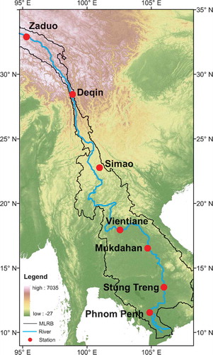
However, a good projection over the LMRB is difficult to achieve because of its complex geography and climate system. The Lancang–Mekong River originates from the Tanggula Mountains in the Tibetan Plateau and stretches down to the South China Sea. Figure 1 shows the complex terrain of the basin including highlands, plains, mountains, hills, and so on, with a great disparity of more than 5000 m in attitude. The elevation directly impacts the spatial distribution of temperature. As a result, the temperature in this basin shows an uneven spatial distribution. Moreover, the LMRB is influenced by the Indian and East Asian summer monsoons, which form a complex climate system and lead to obvious seasonal variation of meteorological elements. These features of the LMRB make it difficult for simulation and projection. Previous studies have mostly used multi-model ensemble results to project the climate change over this basin. For instance, Liu and Xiao (2010) analyzed the projected data of the IPCC multi-model ensemble and found that the regional mean temperature would increase faster in the twenty-first century. Huang et al. (2014) showed an increasing trend of temperature over the whole region. However, these studies focused on the change in mean temperature, which reflects limited information about the climate change in the future. Compared to climatology, the projection of extreme climate events, which needs a higher resolution, is more meaningful in disaster prevention. Yu et al. (2015) explored a future climate projection from the Weather Research and Forecasting (WRF) model. The model results can capture the surface geographic variation, especially in areas of complex topography, such as the edge of the Tibetan Plateau (Yu 2018), which would be a great help in studying the climate features over the LMRB. The objective of this paper is to study the new characteristics of the temperature and extreme temperature events in the twenty-first century over the LMRB.

Figure 1. Elevation map of the Lancang–Mekong River basin (LMRB) (units: m). The blue solid line is the Lancang–Mekong River; the area within the black solid line is the river basin; and the red points are the main stations in the LMRB.

This paper is organized as follows: Section 2 describes the data and methods used in our analyses; Section 3 presents the bias correction and evaluation, and the projection result is also shown in this part; a summary is given in Section 4.

2. Data and methods

The observation product used in this paper is the daily mean temperature from APHRODITE (Asian Precipitation — Highly Resolved Observational Data Integration Toward Evaluation of Water Resources) from 1979 to 2005 with a 0.5° × 0.5° gridded spatial resolution. The simulation was conducted by the WRF model driven by MIROC5 in the context of CMIP5. It included historical (1946–2005) and future projection (2006–2100) simulations under the RCP6 scenario. The computational domain of WRF was (5°–55°N, 70°–160°E), with a spatial resolution of 30 km. Detailed information about the model and experimental design can be found in Yu et al. (2015). In order to allow comparison with the observations, the model results were interpolated to a 0.5° × 0.5° grid using bilinear interpolation. The geographic region focused upon in this paper is (9°–35°N, 95°–108°E).

The method of non-parametric quantile mapping using robust empirical quantiles (RQUANT) was used to correct the bias of simulated temperature. This method has been proven effective by Han et al. (2018). The calculation in this paper uses the R package named qmap (Gudmundsson et al. 2012). The observed temperature and simulated temperature in the reference period were used to build a transfer function to correct the model data during the validation period. The reference period in this paper is from 1979 to 1995 and the validation period is from 1996 to 2005.

3. Results

3.1 Model evaluation

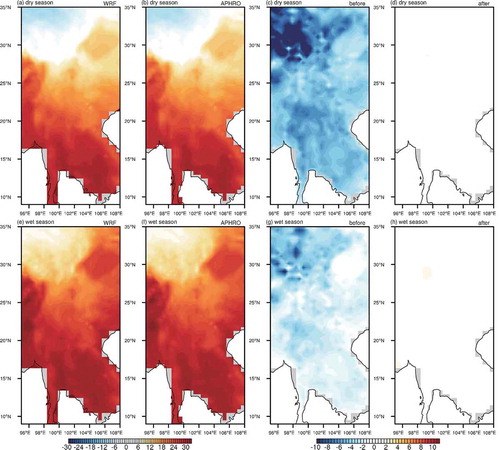
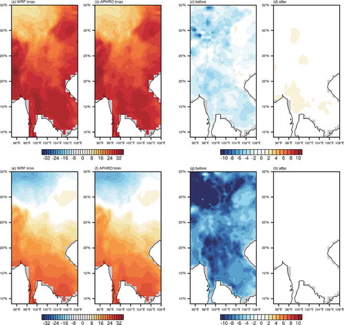
The LMRB is affected by the Indian and East Asian summer monsoons, which leads to two seasons – namely, the wet season from May to October and the dry season from November to April (Lacombe, Smakhtin, and Hoanh 2013). The temperature in these two seasons is analyzed separately because of their distinct features. Figure 2(c,d,g,h) show the bias of simulated temperature before and after correction during the validation period. The simulated temperature is much lower than observation, especially in the northern basin, and the bias is larger in the dry season. After correction, the bias is controlled within ±0.5°C, meaning that RQUANT has a good effect on correcting mean temperature. It can be seen from Figure 2(a,b,e,f) that the seasonal mean temperature from simulation after correction shows the same spatial feature as observation, being higher in the south and lower in the north, and the temperature in the wet season is higher than that in the dry season, indicating that the model simulation after correction can reproduce the special distribution.

Figure 2. Spatial distributions of mean temperature in the (a–d) dry and (e–h) wet season in 1996–2005: (a, e) model simulation; (b, f) APHRODITE; (c, g) biases; (d, h) bias after correction (units: °C).

Using the simulated temperature after correction, the trend of seasonal mean temperature is compared between simulation and observation. According to APHRODITE, the temperature shows an upward trend from 1986 to 2005 at rates of 0.42°C/10 yr in the dry season and 0.18°C/10 yr in the wet season. The model captures the warming trend with a rate of 0.49°C/10 yr in the dry season and a numerically larger rate of 0.28°C/10 yr in the wet season. This indicates that the model is credible in simulating the trend of mean temperature.

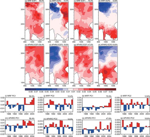
The spatial and temporal characteristics of temperature from simulation and observation are further analyzed using the empirical orthogonal function (EOF). We compare the first two modes whose proportions add up to more than 50% from the corrected simulation results with observation in 1986–2005. It can be seen from Figure 3(e,g) that the dominant feature in both seasons is an all-area consistent increase according to the observation. The second mode is an east-to-west opposite phase in the dry season and a south-to-north opposite phase in the wet season (Figure 3(f,h)). The model results capture the spatial and temporal characteristics and show the same patterns as observation (Figure 3(a–d)), indicating that it is able to simulate the main spatial and temporal variation processes.

Figure 3. The (a–h) spatial distribution and (i–p) time series of EOF1 and EOF2 in the dry season (two left-hand columns) and wet season (two right-hand columns) from simulation and APHRODITE in 1986–2005. The percentages in the upper-right corner represent the proportions explained by EOF1 or EOF2.

The LMRB is under growing threat of extreme temperature in the context of global warming. There has been a distinctly high peak seasonal temperature since 2000 that has influenced the lives of local residents (Mahlstein, Hegerl, and Solomon 2012). Besides, extreme low temperature in this basin can cause yield reductions and harm to agriculture and the economy. Therefore, a credible projection of extreme temperature is important over this region. To validate the effect of RQUANT on the extreme events, we compare the spatial distribution of extreme high and low temperature thresholds – namely, the 95th percentile of the positive-sequence temperature in the wet season and the 5th percentile in the dry season in 1986–2005, from the model before and after the correction with thresholds from APHRODITE. Figure 4(c,g) shows the biases of extreme high and low-temperature thresholds before correction. It is clear that extreme temperature thresholds before correction — especially the extreme low-temperature threshold — deviate considerably compared with observation. RQUANT effectively rectifies the bias of the extreme temperature thresholds, controlling it within ±0.5°C after correction (Figure 4(d,h)). According to Figure 4(a,b,e,f), the spatial characteristics of extreme thresholds from observation and simulation after correction are the same; both are higher in the south and lower in the north, indicating that the model performs well in simulating the extreme temperature thresholds. Based on this result, we selected seven stations in the LMRB (Zaduo, Deqin, Simao, Vientiane, Mukdahan, Stung Treng, and Phnom Penh; the locations of the stations can be seen in Figure 1). The linear interpolation method was used to interpolate the corrected model result to these stations to compare the changing trend of annual days exceeding the extreme high temperature threshold (extreme high-temperature days, EHTD) and annual days lower than the extreme low threshold (extreme low temperature days, ELTD) from WRF after correction with APHRODITE (Table 1). According to APHRODITE, EHTD shows an upward trend except in the middle basin, while ELTD decreases in the whole basin, in 1986–2005. The model after correction reproduces the upward trend of EHTD in Zaduo, Mukdahan, Strung Treng, and Phnom Penh. However, it fails to simulate the downward trend in the middle basin. As for ELTD, the model captures the downward trend in the whole basin. These results suggest that the model simulation performance is better in space than time. It is capable of projecting the spatial distribution of extreme temperature events and is effective at capturing the changing trend of extreme temperature events, especially ELTD. However, caution is needed when applying the model to project the trend of EHTD in the middle basin in the future.

Table 1. Trends of EHTD (extreme high-temperature days) and ELTD (extreme low-temperature days) from model simulation and APHRODITE in 1986–2005 (units: days/10 yr).

	Trend of EHTD		Trend of ELTD
Station	WRF	APHRODITE	WRF	APHRODITE
Zaduo	2.77*	3.41*	−0.37	−5.14*
Deqin	6.44*	−4.36*	−1.37	−0.30
Simao	7.62*	−1.21	−4.19*	−2.94
Vientiane	9.16*	−0.58	−2.85	−2.17
Mukdahan	12.64*	2.99	−4.48*	−3.00
Strung Treng	15.18*	1.85*	−3.45	−5.09*
Phnom Penh	14.28*	7.92*	−3.67*	−5.61*

*Trend showed the significance at the 0.1 level.

Figure 4. Spatial distributions of the (a–d) extreme high and (e–h) low temperature threshold (units: °C) in 1996–2005: (a, e) model simulation; (b, f) APHRODITE; (c, g) biases; (d, h) bias after correction (units: °C).

3.2 Future projection

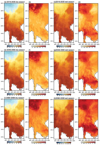
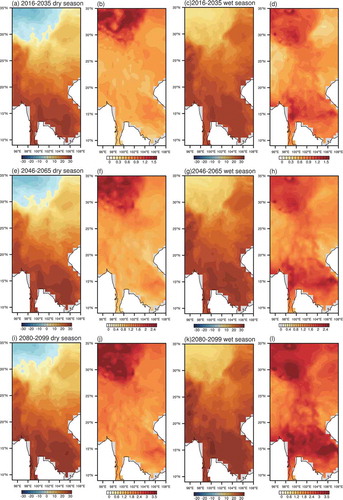
According to the above evaluation, the model performs well in simulating the spatial distribution, temporal, and spatial variation, and extreme temperature events. Based on these results, the future temperature projection in 2016–35, 2046–65, and 2080–99 is analyzed using the model results after correction. Figure 5 shows the spatial distribution of seasonal mean temperature in the future and its difference from the historical period (1986–2005). The spatial distribution of temperature over the LMRB still remains in the original state — namely, higher in the south and lower in the north, and higher in the wet season and lower in the dry season, but with a distinct warming. It can be seen from Figure 5(b,d,f,h,j, l) that the warming in the dry season is most intense in the northern high-altitude area. During the wet season, the warming in the northern high-altitude area is also serious, but the temperature increases greatly in the southern basin too. The warming in the southern basin is more intense in the wet season than in the dry season, which is different from other regions of the world. The above variation is most obvious during 2080–99. Compared to the rest of the domain, the warming is slower in the middle basin.

Figure 5. Spatial distribution of the seasonal mean temperature (first and third columns) and the differences (second and fourth columns) compared with the historical period in the dry season (two left-hand columns) and the wet season (two right-hand columns) in 2016–35 (upper panels), 2046–65 (middle panels), and 2080–99 (lower panels) (units: °C).

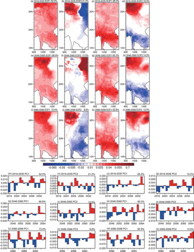
Figure 6 shows the first two spatial modes and temporal series of temperature in the future. The dominant feature of an all-area consistent trend remains the same, as in the historical period. The proportion explained by EOF1 is more than 50% and becomes more significant over time. Combined with the time series (Figure 6(m,q,u)), it shows a weak upward trend in the dry season during 2016–35. Then, the uptrend becomes more obvious in 2046–65, but thereafter fluctuates without a clear trend in 2080–99. In the wet season, the uptrend is obvious in 2016–35 and 2046–65, but changes to a fluctuation without an obvious trend in 2080–2099 (Figure 6(o,s,w)). In the dry season, the second mode (EOF2) shows an east-to-west opposite phase in the northern basin in 2016–35. In 2046–65, it changes to a north-to-south opposite phase that is different from the historical period. In 2080–99, it turns back to a north-to-south opposite phase, but the center of variation moves to the southern basin (Figure 6(d,f,j)). In the wet season, EOF2 shows an opposite between north and south as in the historical period (Figure 6(d,h,l)). Combined with the time series, the temperature in 2016–35 changes from a negative to a positive phase, which indicates that temperature increases in the northern basin and decreases in the southern basin. In 2045–65, the time series of EOF2 changes to a fluctuation without an obvious trend. In 2085–99, as in 2016–35, it shows an upward trend in the time series of EOF2.

Figure 6. The (a–l) spatial distribution and (m–x) time series of EOF1 and EOF2 in the dry season (two left-hand columns) and wet season (two right-hand columns) from simulation in 2016–35, 2046–65, and 2080–99. The percentages in the upper-right corners represent the proportions explained by EOF1 or EOF2.

With the increase in global warming, the features of extreme temperature events will also change in the future. For comparison, the 95th percentile of the positive-sequence temperature in the wet season and the 5th percentile in the dry season during 1986–2005 are again used as the extreme high- and low-temperature thresholds. In order to explore the speed of the variation in EHTD and ELTD at each stage in the future, the differences between the average of the latter period and the average of the former period were calculated at seven stations. It can be seen from Table 2 that EHTD increases in the whole basin and the variation is more intense in the south. EHTD increases most in 2080–99 over the whole region, which echoes the temperature change. As for ELTD, it shows an obvious decrease in the whole region and it changes most in 2016–35 and least in 2046–65. In 2016–35 and 2046–65, the variation is more obvious in the northern basin, but in 2080–99 the decrease is more intense in the middle basin. These features indicate that the warming will be more serious in the future and 2080–99 is a high-incidence period of EHTD. Therefore, the government should be vigilant and make corresponding measures to mitigate disaster risks in advance.

Table 2. Difference between mean EHTD (extreme high-temperature days) and ELTD (extreme low-temperature days) in 2016–35 and 1986–05 (left column), between 2046–65 and 2016–35 (middle column), and between 2080–99 and 2046–65 (right column) (units: day).

	EHTD			ELTD
Station	2016–35	2046–65	2080–99	2016–35	2046–65	2080–99
Zaduo	10.54	12.40	23.73	−5.10	−1.61	−1.16
Deqin	18.58	17.10	32.10	−4.59	−2.20	−1.58
Simao	18.94	24.24	44.73	−4.56	−0.79	−2.58
Vientiane	20.63	24.09	46.93	−4.36	−1.23	−2.83
Mukdahan	20.84	26.43	43.44	−4.20	−0.73	−3.18
Stung Treng	21.74	37.28	54.79	−4.15	−0.80	−2.58
Phnom Penh	19.34	44.99	62.73	−4.36	−0.71	−2.29

4. Conclusions and discussion

This paper first evaluates the simulated temperature corrected by the RQUANT method over the LMRB. According to the results, the model performs well in simulating the spatial distribution characteristics of mean temperature as well as the extreme high- and low-temperature events and their changing trends. In addition, according to EOF results, it can capture the main characteristics of spatial variation.

Based on the above evaluation results, the projection of temperature and extreme temperature events indicates that, in the future, the temperature in the LMRB will maintain the original characteristics of spatial distribution and keep increasing. From the perspective of spatial distribution, the warming in the northern basin will be more intense in the dry season, but the warming in the middle and southern basin will be more intense in the wet season. From the perspective of temporal variation, the increase in temperature will become most obvious in 2080–99. The dominant feature of the spatial variation will still exhibit an all-area consistent pattern. The second mode in the wet season will keep a west-to-east opposite phase in the future, as before. In the dry season, the second mode will change from an east-to-west opposite phase to a north-to-south opposite phase in 2046–65 and return to the antiphase distribution between east and west in 2080–99. As for the extremes, EHTD will occur more often, especially in the downstream, and will become most frequent in 2080–99. ELTD is projected to decline in the whole basin.

It is known that temperature variation— especially extreme temperature events — can have a direct impact on agricultural production, water resource management, human mortality, and so on. Moreover, it will also cause precipitation changes through increasing water evaporation, which may lead to drought, flooding, and other disasters (Hu, Maskey, and Uhlenbrook 2013). But how will the precipitation over the LMRB change in the future? And will the characteristics of extreme events be different? These questions also merit further investigation.

Disclosure statement

No potential conflict of interest was reported by the authors.

Additional information

Funding

This work was supported by the External Cooperation Program of Bureau of International Co-operation, Chinese Academy of Sciences [grant number GJHZ1729] and the Key Program of the Natural Science Foundation of Yunnan Province of China [grant number 2016FA041].

References

- Diffenbaugh, N. S., D. Singh, J. S. Mankin, D. E. Horton, D. L. Swain, D. Touma, A. Charland, et al. 2017. “Quantifying the Influence of Global Warming on Unprecedented Extreme Climate Events.” Proceedings of the National Academy of Sciences of the United States of America 114 (19): 4881–4886. DOI:10.1073/pnas.1618082114.
- Gudmundsson, L., J. B. Bremnes, J. E. Haugen, and T. E. Skaugen. 2012. “Technical Note: Downscaling RCM Precipitation to the Station Scale Using Statistical Transformations - A Comparison of Methods.” Hydrology and Earth System Sciences 16: 3383–3390.
- Han, Z. Y., Y. Tong, X. J. Gao, and Y. Xu. 2018. “Correction Based on Quantile Mapping for Temperature Simulated by the RegCM4.” Climate Change Research (In Chinese) 14: 331–340.
- Hu, Y. R., S. Maskey, and S. Uhlenbrook. 2013. “Downscaling Daily Precipitation over the Yellow River Source Region in China: A Comparison of Three Statistical Downscaling Methods.” Theoretical and Applied Climatology 112 (3–4): 447–460.
- Huang, Y., F. Y. Wang, Y. Li, and T. J. Cai. 2014. “Multi-Model Ensemble Simulation and Projection in the Climate Change in the Mekong River Basin. Part I: Temperature.” Environmental Monitoring and Assessment 186 (11): 7513–7523.
- IPCC. 2014. Climate Change 2014: Synthesis Report. Contribution of Working Groups I, II and III to the Fifth Assessment Report of the Intergovernmental Panel on Climate Change, 151. Geneva: IPCC. Edited by Core Writing Team, R. K. Pachauriand L. A. Meyer.
- Lacombe, G., V. Smakhtin, and C. T. Hoanh. 2013. “Wetting Tendency in the Central Mekong Basin Consistent with Climate Change-Induced Atmospheric Disturbances Already Observed in East Asia.” Theoretical and Applied Climatology 111 (1–2): 251–263.
- Liu, B., and Z. N. Xiao. 2010. “Observed (1951–2008) and Projected (2010–2099) Climate Change in the Lancang River Basin.” Advances in Climate Change Research (In Chinese) 6: 170–174.
- Ma, Z. F., J. Liu, S. Q. Zhang, W. X. Chen, and S. Q. Yang. 2013. “Observed Climate Changes in Southwest China during 1961–2010.” Advances in Climate Change Research 4: 0–40.
- Mahlstein, I., G. Hegerl, and S. Solomon. 2012. “Emerging Local Warming Signals in Observational Data.” Geophysical Research Letters 39: L21711.
- Manton, M. J., P. D. Marta, M. R. Haylock, K. J. Hennessy, N. Nicholls, L. E. Chambers, and D. A. Collins. 2001. “Trends in Extreme Daily Rainfall and Temperature in Southeast Asia and the South Pacific: 1961–1998.” International Journal of Climatology 21 (3): 269.
- Rahmstorf, S., and D. Coumou. 2011. “Increase of Extreme Events in a Warming World.” Proceedings of the National Academy of Sciences of the United States of America 108 (44): 17905–17909.
- Thirumalai, K., P. N. Dinezio, Y. Okumura, and C. Deser. 2017. “Extreme Temperatures in Southeast Asia Caused by El Niño and Worsened by Global Warming.” Nature Communications 8: 15531.
- Wu, F. F., X. Wang, Y. P. Cai, Z. F. Yang, and C. H. Li. 2012. “Spatiotemporal Analysis of Temperature-Variation Patterns under Climate Change in the Upper Reach of Mekong River Basin.” The Science of the Total Environment 427–428: 208–218.
- Yu, E. T. 2018. “A Warmer, Wetter and Less Windy China in the Twenty-First Century as Projected by A Nested High-Resolution Simulation Using the Weather Research and Forecasting (WRF) Model.” Asia-Pacific Journal of Atmospheric Sciences 55: 53–74.
- Yu, E. T., J. Q. Sun, H. P. Chen, and W. L. Xiang. 2015. “Evaluation of A High-Resolution Historical Simulation over China: Climatology and Extremes.” Climate Dynamics 45: 2013–2031.