Joint optimization of production lot-sizing and condition-based maintenance in an imperfect production process with dependent indicators

ABSTRACT

This paper addresses the integrated optimization of the economic manufacturing quantity and the condition-based maintenance policy of a deteriorating manufacturing system. The considered facility produces a single type of product and is inspected at the end of each production run. Upon inspection, two dependent indicators are revealed: one implies whether the production process is in control or not and the other one represents the deterioration level of the facility. The dependence between the two indicators is that whenever the facility deterioration exceeds a pre-determined level, the system becomes more vulnerable such that the production process may switch to the out-of-control state. In the out-of-control state, a proportion of defective items is fabricated. Considering the inter-dependencies between production process and machine degradation, this paper develops an integrated production and maintenance model to minimize the overall cost. The expected cost rate in the long run is taken as the objective function to assess the proposed model, where the joint optimization of the lot-sizing and the maintenance policy is developed. The problem is formulated in the context of a semi-Markov decision process and solved with the successive approximation method. A numerical example is given to illustrate the applicability of the proposed model.

KEYWORDS:

• Economic manufacturing quantity
• condition-based maintenance
• dependent indicators
• semi-Markov decision process

1. Introduction

With the development of the scientific and technological innovations, manufacturing process is changing rapidly to meet emerging demands. From the perspectives of manufacturers, they always intend to maximizing their profits by meeting the customer demand, preventing the shortage loss and controlling the inventory budget. The economic manufacturing quantity (EMQ) models (Chakraborty & Giri, 2012; Hadidi et al., 2012; Jiang & Farr, 2007; Park, 2021; Sana & Chaudhuri, 2010; Sarkar et al., 2014; Sicilia et al., 2014) have been proposed to address these objectives. In the classical EMQ models, a common assumption is that the facility will never deteriorate or fail during a production run. Therefore, the quality control process and the maintenance planning are regarded as independent events such that the corresponding strategies are developed separately.

However, in reality, even the sophistical facility with high reliability and superduty productivity may deteriorate due to the usage and aging. The facility deterioration will lead to decreased performance with lower production rate, unsatisfied product quality (Hong-Fwu & Chen, 2018), etc. In addition, a sudden system failure and the corresponding maintenance may cease the production run and derange the production schedule. Glock (2012) and Glock et al. (2014) have stated that the deterioration of the machine had a significant effect on the product quality and the inventory cost. Hence, it is essential to jointly consider the EMQ and the maintenance policies (Abdur Rahim & Ben-Daya, 2012; Chakraborty & Giri, 2014; Ouaret et al., 2018; Sarkar et al., 2010).

With respect to the maintenance planning (Qiu et al., 2019; Scarf, 2007; Wang et al., 2020), condition-based maintenance (CBM) has received increasing attention in recent years. It allows to make maintenance decisions based on the sensor information with respect to the health condition of the system, especially when failure data are rare in highly reliable mechanical systems nowadays. In this framework, various models have been proposed to investigate the maintenance strategy, where the maintenance cost and the system availability are the most commonly used assessment criteria. Various system configurations, deterioration characteristics, inspection policies and maintenance criteria have been studied (Hu & Chen, 2020; Zhang et al., 2020, Zhang et al., 2020). The influence of the CBM on product scheduling and the integrated optimization of the EMQ and CBM have been investigated by several researchers. Boukas and Liu (2001) addressed the production and maintenance problem of a failure-prone manufacturing system which had three states following a continuous-time Markov chain. The optimal production and maintenance rates were discussed. Jafari and Makis (2019) also utilized a continuous-time Markov chain with three states to model a production system. By assuming that the non-failure states were partially observable, they derived the optimal Bayesian control policy in the semi-Markov decision process (SMDP) framework. Sloan and Shanthikumar (2000) developed a Markov decision process model to determine the maintenance and production schedules of a multiple-product, single-machine system. The impact of the machine condition on the yield of each type of the products was examined. Peng and van Houtum (2016) modelled the deterioration of the machine by a Gamma process and took the preventive maintenance (PM) threshold and the lot-sizing as the decision parameters in the evaluation of the joint optimization problem. Cheng et al. (2018) combined the health condition of the machine and the quality information in determining the optimal maintenance policy.

It can be observed that the above-mentioned integrated optimization of the EMQ and CBM models have considered only one indicator representing the facility condition. In effect, multiple dependent indicators can be utilized in the condition monitoring of the system. For instance, Mercier et al. (2012) measured the deterioration of the railway track geometry by a bivariate Gamma process which took the longitudinal and transversal levelling indicators into consideration. In the oil and gas production system, a throttle valve may fail due to the corrosion or a sudden failure (Zhang, 2018). Jafari and Makis (2015) presented an example: the level of metal particles in an engine oil or a vibration monitoring level the machine deterioration may indicate the deterioration of the system. They utilized a proportional hazards model to incorporate the covariates into the hazard rate function. Similar considerations can be found in Zheng et al. (2021) where decisions were made based on both the system deterioration and the system age. Some studies examine production systems with multiple components. In this scenario, the state of each component can be regarded as an indicator of the system state. Jafari and Makis (2016) and Zheng and Zhou (2022) considered a production facility with two components. However, there is little work considering multiple indicators in the framework of the joint optimization of the EMQ and CBM models.

In this study, we will consider the system that is described by two dependent indicators: one is modelled by a continuous state process, representing the deterioration of the facility, and the other one possesses only two observable states, indicating whether the production process is in control or not. Whenever the facility deterioration exceeds a pre-determined level, the system becomes more vulnerable and the production process may transfer to the out-of-control state. The facility is inspected at the end of each production run such that the true state of the system can be obtained, which contains the deterioration level and the in-control/out-of-control information.

Generally, the quality of the product depends on the production process, and non-confirming quality products may occur whenever the production procedure shifts from its in-control state to the out-of-control state. Rosenblatt and Lee (1986) assumed that the system shifted to the out-of-control process with a certain time period where the produced items became defective. Sankar Sana et al. (2007) investigated an imperfect production process by assuming the mixture of the productions of the perfect and imperfect items, where imperfect items were sold at a reduced price. Malik and Sarkar (2020) considered a multi-product imperfect production system, where the defective rate was assumed to be a constant and defective items were abandoned. Under the budget, space, reliability and demand constraints, the total expected profit was selected as the objective function to assess the model. In this paper, we also consider that whenever the production process shifts to the out-of-control process, defective items are produced with a probability which depends on the system deterioration level: whenever the deterioration indicator exceeds a predefined threshold, the defective rate increases. Defective product can be repaired to the perfect state before sale. The defective rate on the joint optimization of the EMQ and CBM will be discussed in detail in the following context.

In a nutshell, for the decision-maker, when the production facility possesses two indicators and defective items are related to the system deterioration, how to determine the optimal production and maintenance scheduling? This study intends to address the problem as an integrated optimization of the production lot-sizing and CBM policy. The expected cost occurred during the production, and maintenance per unitary time is taken to implement the policy. We cast the problem into a semi-Markov decision process and solved it with the successive approximation method. The main contributions of this study are the following:

• A joint optimization of the production and conditional-based maintenance policy is studied.

• Two dependent indicators are employed to represent the production and system conditions.

• The lot-sizing and the PM threshold are jointly optimized by minimizing the expected cost per unitary time in the infinite horizon.

The rest of the paper is organized as follows: In Section 2, the problem statement, general model assumptions and system characteristics are given. In Section 3, the problem is formulated in the framework of the semi-Markov decision process. Section 4 deals with the derivation of the expected maintenance cost where the successive approximation method is proposed to solve the problem. The corresponding sensitivity analysis is also illustrated to show the applicability of the model. Finally, we make the conclusion in Section 5.

2. Model description

Consider a manufacturing system that produces a single type of product with the lot size $Q$ in each production run. The production and demand rates are, respectively, $p$ and $d$, $p>d.$ The facility is subjected to deterioration, and its state is described by two dependent indicators. Indicator 1 has only two discrete observations representing whether the production process is in control or not. Indicator 2 is modelled by a monotonic, continuous process representing the degradation level of the system. Upon inspection, both of the two indicators can be perfectly observed. Define $X_t^{(1)}$ as the value of indicator 1 with

$X_t^{(1)}=\left\{\begin{array}{cc}0,& \mathrm{i}\mathrm{f}\mathrm{t}\mathrm{h}\mathrm{e}\mathrm{p}\mathrm{r}\mathrm{o}\mathrm{d}\mathrm{u}\mathrm{c}\mathrm{t}\mathrm{i}\mathrm{o}\mathrm{n}\mathrm{p}\mathrm{r}\mathrm{o}\mathrm{c}\mathrm{e}\mathrm{s}\mathrm{s}\mathrm{i}\mathrm{s}\mathrm{i}\mathrm{n}-\mathrm{c}\mathrm{o}\mathrm{n}\mathrm{t}\mathrm{r}\mathrm{o}\mathrm{l}\mathrm{a}\mathrm{t}t,\\ 1,& \mathrm{i}\mathrm{f}\mathrm{t}\mathrm{h}\mathrm{e}\mathrm{p}\mathrm{r}\mathrm{o}\mathrm{d}\mathrm{u}\mathrm{c}\mathrm{t}\mathrm{i}\mathrm{o}\mathrm{n}\mathrm{p}\mathrm{r}\mathrm{o}\mathrm{c}\mathrm{e}\mathrm{s}\mathrm{s}\mathrm{i}\mathrm{s}\mathrm{o}\mathrm{u}\mathrm{t}-\mathrm{o}\mathrm{f}-\mathrm{c}\mathrm{o}\mathrm{n}\mathrm{t}\mathrm{r}\mathrm{o}\mathrm{l}\mathrm{a}\mathrm{t}t.\end{array}\right.$

Let $T$ be the sojourn time that the production is in-control from its initial producing time with the cumulative density function (CDF) $F$ and probability density function (PDF) $f$, respectively. Let $X_t^{(2)}$ be the deterioration of the system which is modelled by a homogeneous Gamma process with probability density function

(1) ${\psi }_{\alpha t,\beta }(x)=\frac{{\beta }^{\alpha t}}{\mathrm{\Gamma }(\alpha t)}{x}^{\alpha t-1}{e}^{-\beta x},x\ge 0,$(1)

where $\mathrm{\Gamma }$ is a Gamma function with

$\mathrm{\Gamma }(\alpha t)={\int }_0^{\mathrm{\infty }}{v}^{\alpha t-1}{e}^{-v}\mathrm{d}v.$

Thus, the degradation of the system is a monotonic process. Let ${\sigma }_y$ be the first passage time corresponding to threshold $y$, $y\ge 0$, which is defined as

${\sigma }_y=\mathrm{i}\mathrm{n}\mathrm{f}\{t\ge 0,X_t^{(2)}\ge y\}.$

Let $G_{{\sigma }_y}(t)$ be the distribution function of ${\sigma }_y$, then

(2) $G_{{\sigma }_y}\left(t\right)=\mathbb{P}\left({\sigma }_y\le t\right)=\mathbb{P}\left(X_t^{\left(2\right)}\ge y\right)=\frac{\mathrm{\Gamma }\left(\alpha t,y\beta \right)}{\mathrm{\Gamma }\left(\alpha t\right)},$(2)

where $\mathrm{\Gamma }(\cdot ,\cdot )$ is the incomplete Gamma function with

$\mathrm{\Gamma }(\alpha ,x)={\int }_x^{\mathrm{\infty }}{z}^{\alpha -1}{e}^{-z}\mathrm{d}z.$

The corresponding density function of ${\sigma }_y$ is defined as $g_{{\sigma }_y}(t).$

The system failure time is defined as the time epoch whenever the degradation level firstly exceeds the pre-determined threshold $L,L>0.$ Whenever the system transfers to the out-of-control state, it can still fulfill its functionality but with imperfect performance by producing defective products. Besides, the two indicators are dependent: the system may shift to the out-of-control state from the in-control-state with probability $\mu$ if its deterioration level exceeds $M_s$, $0<M_s<L$, $\mu \in [0,1]$. Thus, we have introduced two dependent indicators representing the facility state. One is discrete with only two states indicating whether the production process is in control or not. The other one is described by a Gamma process with non-decreasing trajectories and pure jump characteristic. As in the classical EMQ model, assume that the production run with product quantity $Q$ is $\tau$ and the system is inspected at the end of each run. If the inspection result shows that the system is in a good working condition, no maintenance action will be implemented, and the machine will experience an idle time of period $(p-d)\tau /d$. For simplicity, assume that both the control process and the degradation suspend during the idle period. The production process starts over whenever the inventory goes back to 0.

3. Maintenance model

To ensure the production quality and to avoid the economic loss, a maintenance policy will be employed to prevent the system from failure. This section discusses the CBM model within the manufacturing process. As mentioned before, the system is inspected at the end of each production phase. Upon inspection, we can observe the two system indicators as presented in Section 2. As the system sojourn time in the in-control state follows a generic distribution, we need to record the time elapsed in the in-control phase. Define $(S_t,Y_t)$ as the tuple with $S_t$ representing the passing time in the in-control state since its last adjustment and $Y_t$ representing the deterioration level at time $t$. The costs and the maintenance policy are given as follows:

• The holding cost of each item per unitary time $c_h,c_h\ge 0.$

• At the end of each production run, the system is inspected with cost $c_I$ and the inspection time is negligible, $c_I\ge 0$.

• Whenever no system failure occurs, if the system is found in the ‘out-of-control’ state, it is adjusted to the ‘in-control’ state with cost $c_{p1}$ and $t_{p1}$ time units, $c_{p1}\ge 0,$ $t_{p1}\ge 0.$

• Whenever the degradation level of the system exceeds a predefined threshold $M$, it is restored to the as-good-as-new state $(0,0)$ with cost $c_p$ and time units $t_p$, $c_p\ge c_{p1}$, $t_p\ge t_{p1}.$

• The system fails whenever its degradation level exceeds a predefined level $L$. The failure is self-announcing, and corrective maintenance is executed immediately with cost $c_f$ and time units $t_f$. The system is restored to the as-good-as-new state $(0,0)$ with the corrective maintenance, $c_f\ge c_p$, $t_f\ge t_p.$

• Besides the maintenance cost, economic loss may occur due to the restoration of the defective items and the time depletion caused by the maintenance actions. The loss cost is $c_l$ per unitary time. The product defectiveness occurs whenever the production process is out of control, $c_l>0$. The defective rate at time $t$ depends on the deterioration state of the system. The defective rate is larger with severe deterioration. Here, we suppose that

$r_t=\left\{\begin{array}{cc}{r}_0,& X_t^{(1)}=1,Y_t\le M_s,\\ r_1,& X_t^{(1)}=1,Y_t>M_s,\\ 0,& \mathrm{O}\mathrm{t}\mathrm{h}\mathrm{e}\mathrm{r}\mathrm{w}\mathrm{i}\mathrm{s}\mathrm{e}.\end{array}\right.$

• The restoration cost of each defective item is $c_d$, $c_d>0$.

• Set-up cost $c_s$, $c_s>0$, occurs after a corrective/preventive maintenance action due to the material/repairment preparation, etc.

Figures 1–3 show three scenarios that the system is intervened due to maintenance actions. In Figure 1, it is seen that during the manufacturing process, the control process and the system degradation level are inspected at the end of each production run. Whenever the self-announcing system failure occurs, meaning that the degradation level firstly arrives or exceeds the failure threshold $L$, the system is correctively renewed. Otherwise, if the system degradation level is between the preventive maintenance threshold $M$ and the failure threshold $L$ at the end of a production run, the system is preventively renewed, which is illustrated in Figure 2.

Figure 1. Illustration of corrective maintenance.

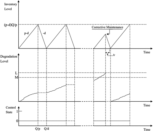
Figure 2. Illustration of preventive maintenance.

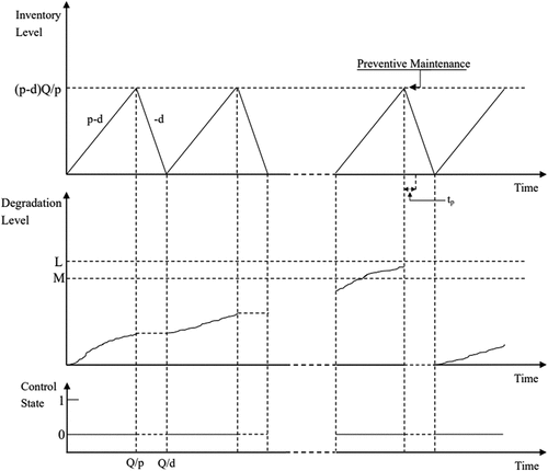
Figure 3. Illustration of adjustment of the control state.

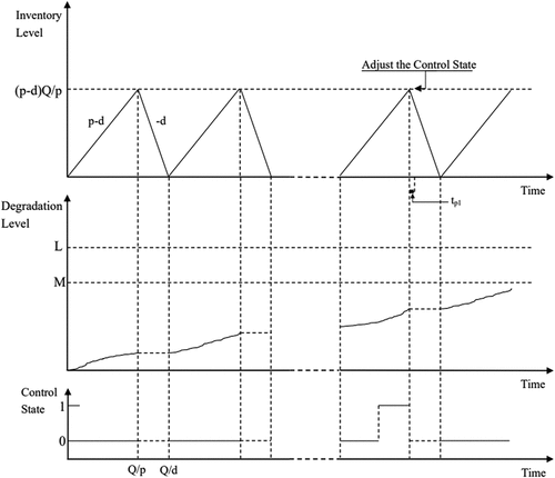
In Figure 3, the intervention also occurs upon the inspection, where the mechanical condition of the system is good with degradation level lower than $M$, but it is found in the out-of-control state. Hence, the manufacturing process is adjusted to the in-control process with degradation level remains unchanged. Our objective is to jointly optimize the production loss $Q$ and the condition-based maintenance threshold $M$ to achieve the minimization of the expected maintenance cost rate $C_{\mathrm{\infty }}\left(Q^{\ast },M^{\ast }\right)$. The problem is formulated in the framework of a semi-Markov decision process. The transition kernel is presented in detail in the following discussions.

3.1. The transition kernel

With consideration of the maintenance actions, the system state can be classified as follows.

• state $(0,0)$: the system is in its as-good-as-new state,

• state $(k,y)$: the system stays in the in-control state at the $k$th production run since its last adjustment, and the degradation level of the system is $y$, $k\ne 0,0<y\le M,$

• state $(P{M}_1,y)$: the control process is adjusted, $0<y\le M$,

• state $(0,y)$: the system restores to the in-control process with age 0 and the degradation level of the system is $y,0<y\le M$,

• state $P{M}_s$: the system is preventively maintained.

The above states contain all the scenarios that can be observed upon the inspection. The transition kernels among them can be further calculated. Let $p_{A\to B}$ be the transition kernel that the system state transfers from state $A$ to state $B$. Whenever the system stays in $(k,y)$, it is possible that at the next inspection, the system is still in control, and the deterioration level does not exceed $M$. Under this scenario, we have that

$p_{(k,y)\to (k+1,y^{\prime })}=\mathbb{P}(T>(k+1)\tau ,Y_{(k+1)\tau }\in y^{\prime }|T>k\tau ,Y_{k\tau }=y)\bar{\mu }{I}_{\{y\le M_s,y^{\prime }>M_s\}},$

(3) $+\mathbb{P}(T>(k+1)\tau ,Y_{(k+1)\tau }\in y^{\prime }|T>k\tau ,Y_{k\tau }=y)$(3)

$\times (I_{\{y\le M_s,y^{\prime }\le M_s\}}+I_{\{y\ge M_s,y^{\prime }\ge M_s\}}),$

$=\frac{\bar{F}((k+1)\tau )}{\bar{F}(k\tau )}{\psi }_{\alpha \tau ,\beta }(y^{\prime }-y)$

$\times (\bar{\mu }{I}_{\{y\le M_s,y^{\prime }>M_s\}}+I_{\{y\le M_s,y^{\prime }\le M_s\}}+I_{\{y>M_s,y^{\prime }>M_s\}}),$

where $\mu$ is the probability that the system shifts to the out-of-control process by a sudden shock whenever the deterioration level firstly exceeds $M_s$. $\bar{\mu }=1-\mu$, $I_A$ is the indicator function with set $A$. Definition of $\psi$ can be found in Equation (1)(1) ${\psi }_{\alpha t,\beta }(x)=\frac{{\beta }^{\alpha t}}{\mathrm{\Gamma }(\alpha t)}{x}^{\alpha t-1}{e}^{-\beta x},x\ge 0,$(1) . $F$ is CDF of the sojourn time of the ‘in-control’ state, $\bar{F}=1-F.$ If the system state shifts to the ‘out-of-control’ process and the degradation level is still within the preventive maintenance threshold such that

$p_{(k,y)\to (P{M}_1,y^{\prime })}=(1-\bar{\mu }\mathbb{P}(T>(k+1)\tau ,Y_{(k+1)\tau }\in y^{\prime }|T>k\tau ,Y_{k\tau }=y))I_{\{y\le M_s,y^{\prime }>M_s\}}$

$+\mathbb{P}(T<(k+1)\tau ,Y_{(k+1)\tau }\in y^{\prime }|T>k\tau ,Y_{k\tau }=y)$

$\times ({\mathit{I}}_{\{y\le M_s,y^{\prime }\le M_s\}}+{\mathit{I}}_{\{y\ge M_s,y^{\prime }\ge M_s\}}),$

(4) $=(1-\bar{\mu }\frac{\bar{F}((k+1)\tau )}{\bar{F}(k\tau )}){\psi }_{\alpha \tau ,\beta }(y^{\prime }-y){\mathit{I}}_{\{y\le M_s,y^{\prime }>M_s\}}$(4)

$+\frac{F((k+1)\tau )-F(k\tau )}{\bar{F}(k\tau )}{\psi }_{\alpha \tau ,\beta }(y^{\prime }-y)({\mathit{I}}_{\{y\le M_s,y^{\prime }\le M_s\}}+{\mathit{I}}_{\{y>M_s,y^{\prime }>M_s\}}).$

In addition, the probability that the system is preventively replaced is

(5) $p_{(k,y)\to P{M}_s}=(G_{{\sigma }_{M-y}}(\tau )-G_{{\sigma }_{L-y}}(\tau )).$(5)

where $G$ has been presented in Equation (2)(2) $G_{{\sigma }_y}\left(t\right)=\mathbb{P}\left({\sigma }_y\le t\right)=\mathbb{P}\left(X_t^{\left(2\right)}\ge y\right)=\frac{\mathrm{\Gamma }\left(\alpha t,y\beta \right)}{\mathrm{\Gamma }\left(\alpha t\right)},$(2) . Similarly, the probability that the system is correctively replaced is

(6) $p_{(k,y)\to (0,0)}=G_{{\sigma }_{L-y}}(\tau ).$(6)

The transition probabilities for the remaining states are

(7) $p_{(P{M}_1,y)\to (0,y)}=1,$(7)

(8) $p_{(P{M}_s)\to (0,0)}=1.$(8)

3.2. Expected sojourn times

Let $T_s$ be the expected sojourn time given the initial state is $s$. Whenever the system state is $s=(k,y)$, meaning that the deterioration level is $y$ at the $k$th production run since the last adjustment of the control process, for any $k\in$, $0\le y\le M$, $T_{(k,y)}$ can be calculated:

(9) $T_{(k,y)}=(\frac{Q}{d}-\tau )I_{\{(k,y)\ne (0,0)\}}+\tau {\bar{G}}_{{\sigma }_{L-y}}(\tau )+{\int }_0^{\tau }(t+\mathrm{m}\mathrm{a}\mathrm{x}(u(t),t_f))\mathrm{d}{G}_{{\sigma }_{L-y}}(t),$(9)

where $u(t)=\frac{p-d}{d}t$. In addition, if $\tau <\frac{d{t}_f}{p-d}$, the integral on the right-hand side can be further given as $(\tau +t_f)G_{{\sigma }_{L-y}}(\tau )-{\int }_0^{\tau }{G}_{{\sigma }_{L-y}}(t)\mathrm{d}t$. Otherwise, it is equal to $\frac{p}{d}\tau G_{{\sigma }_{L-y}}(\tau )-\frac{p-d}{d}{\int }_{\frac{d{t}_f}{p-d}}^{\tau }{G}_{{\sigma }_{L-y}}(t)\mathrm{d}t-{\int }_0^{\tau }{G}_{{\sigma }_{L-y}}(t)\mathrm{d}t$.

Similarly, we have that

(10) $T_{(P{M}_1,y)}=\mathrm{m}\mathrm{a}\mathrm{x}(\frac{Q}{d}-\frac{Q}{p},t_{p1}),$(10)

(11) $T_{P{M}_s}=\mathrm{m}\mathrm{a}\mathrm{x}(\frac{Q}{d}-\frac{Q}{p},t_p).$(11)

3.3. Expected costs

As a first step, the expected number of the defective items is calculated. Let $N_d(k,y)$ be the expected number of defective products during the period that the initial state of the system is $(k,y)$, $k\in$, $0\le y\le M$. If $y>M_s$, then we have:

$N_d(k,y)={\bar{G}}_{{\sigma }_{L-y}}(\tau ){\int }_0^{\tau }{r}_{1}p(\tau -t)\frac{f(t+k\tau )}{\bar{F}(k\tau )}\mathrm{d}t,$

$+{\int }_0^{\tau }{g}_{{\sigma }_{L-y}}(t){\int }_0^t{r}_{1}p(t-v)\frac{f(v+k\tau )}{\bar{F}(k\tau )}\mathrm{d}v\mathrm{d}t,$

$=\frac{r_{1}p}{\bar{F}(k\tau )}({\int }_0^{\tau }{\bar{G}}_{{\sigma }_{L-y}}(\tau )(F(t+k\tau )-F(k\tau ))\mathrm{d}t,$

$+{\int }_0^{\tau }(G_{{\sigma }_{L-y}}(\tau )-G_{{\sigma }_{L-y}}(v))(F(v+k\tau )-F(k\tau ))\mathrm{d}v),$

$=\frac{r_{1}p}{\bar{F}(k\tau )}{\int }_0^{\tau }(1-G_{{\sigma }_{L-y}}(v))(F(v+k\tau )-F(k\tau ))\mathrm{d}v.$

Otherwise, whenever $y\le M_s$, the expected number of the defective items depends on $\mu$, the probability that out-of-control occurs due to the severe deterioration of the system. In this scenario, $N_d(k,y)$ can be represented as

$N_d(k,y)=\frac{r_{0}p}{\bar{F}(k\tau )}{\bar{G}}_{{\sigma }_{M_s-y}}(\tau ){\int }_0^{\tau }(F(t+k\tau )-F(k\tau ))\mathrm{d}t,$

$+\frac{p}{\bar{F}(k\tau )}{\int }_0^{\tau }{g}_{{\sigma }_{M_s}-y}(t){\bar{G}}_{{\sigma }_L-{\sigma }_{M_s}}(\tau -t)$

$\times (r_0{\int }_0^{t}F(v+k\tau )\mathrm{d}v-r_{0}tF(k\tau )+r_1\bar{\mu }{\int }_t^{\tau }F(v+k\tau )\mathrm{d}v+r_1\mu (\tau -t)\bar{F}(k\tau ))\mathrm{d}t,$

$+\frac{p}{\bar{F}(k\tau )}{\int }_0^{\tau }{\int }_t^{\tau }{g}_{{\sigma }_L-{\sigma }_{M_s}}(\theta )g_{{\sigma }_{M_s}-y}(t)$

$\times (r_0{\int }_0^{t}F(v+k\tau )\mathrm{d}v-r_{0}tF(k\tau )+r_1\bar{\mu }{\int }_t^{\theta }F(v+k\tau )\mathrm{d}v+r_1\mu (\theta -t)\bar{F}(k\tau ))\mathrm{d}t.$

Let $A_{(k,y)}$ be the expected cost with system initial state $(k,y)$ until the next decision time epoch without consideration of the holding cost in the idle period, then

$A_{(k,y)}=c_s+{\bar{G}}_{{\sigma }_L-y}(\tau )(c_i+c_h{\int }_0^{\tau }(p-d)t\mathrm{d}t)+c_d{N}_d(k,y)$

$+{\int }_0^{\tau }(c_f+c_h({\int }_0^t(p-d)\theta \mathrm{d}\theta +{\int }_0^{u(t)}(p-d)t-\theta d\mathrm{d}\theta )+c_{l}d\times \mathrm{m}\mathrm{a}\mathrm{x}(t_f-u(t),0))\mathrm{d}{G}_{{\sigma }_L-y}(t)$

$=\left\{\begin{array}{cc}{c}_s+{\bar{G}}_{{\sigma }_L-y}(\tau )(c_i+\frac{(p-d){\tau }^2{c}_h}{2})+(c_f+c_{l}d{t}_f)G_{{\sigma }_L-y}(\tau )& \hspace{0.17em}\\ +\frac{p(p-d)c_h}{2d}{\int }_0^{\tau }{t}^2\mathrm{d}{G}_{{\sigma }_L-y}(t)+c_d{N}_d(k,y),& \mathrm{i}\mathrm{f}\tau <\frac{d{t}_f}{p-d},\\ c_s+{\bar{G}}_{{\sigma }_L-y}(\tau )(c_i+\frac{(p-d){\tau }^2{c}_h}{2})+c_f{G}_{{\sigma }_L-y}(\tau )+\frac{p(p-d)c_h}{2d}{\int }_0^{\tau }{t}^2\mathrm{d}{G}_{{\sigma }_L-y}(t)& \hspace{0.17em}\\ +c_l(p-d)\tau G_{{\sigma }_L-y}(\tau )-c_l(p-d){\int }_{\frac{d{t}_f}{p-d}}^{\tau }{G}_{{\sigma }_L-y}(t)\mathrm{d}t+c_d{N}_d(k,y)& \mathrm{O}\mathrm{t}\mathrm{h}\mathrm{e}\mathrm{r}\mathrm{w}\mathrm{i}\mathrm{s}\mathrm{e}.\end{array}\right.$

Let $C_{\mathbf{s}}$ be the expected cost occurred with the system initial state $s$ until the next decision epoch, then

(12) $C_{(0,0)}=A_{(0,0)}.$(12)

(13) $C_{(k,y)}=\frac{{(p-d)}^2{\tau }^2}{2d}{c}_h+A_{(k,y)}.$(13)

Besides, the cost associated with the adjustment of the control process when the system degradation level is $y$ can be obtained as:

(14) $C_{(P{M}_1,y)}=c_{p1}+c_{l}d\mathrm{m}\mathrm{a}\mathrm{x}(t_{p1}-(\frac{Q}{d}-\tau ),0)+{\int }_0^{\frac{Q}{d}-\frac{Q}{p}}(c_h(p-d)Q/p-td)\mathrm{d}t.$(14)

Similarly, given that the system is to be preventively renewed, the expected cost is

(15) $C_{P{M}_s}=c_p+c_{l}d\mathrm{m}\mathrm{a}\mathrm{x}(t_p-(\frac{Q}{d}-\tau ),0)+{\int }_0^{\frac{Q}{d}-\frac{Q}{p}}(c_h(p-d)Q/p-td)\mathrm{d}t.$(15)

We have derived all the elements corresponding to the semi-Markov decision process. To obtain the expected cost rate of the system in the long run, define ${\pi }_s$ as the stationary distribution of the corresponding embedded Markov chain of the SMDP, we have

(16) ${\pi }_{(0,0)}={\pi }_{(0,0)}{p}_{(0,0)\to (0,0)}+\sum _{k\in \mathbb{N}}{\int }_0^M{\pi }_{(k,y)}{p}_{(k,y)\to (0,0)}\mathrm{d}y+{\pi }_{P{M}_s},$(16)

${\pi }_{\left(k,y\right)}={\pi }_{\left(0,0\right)}{p}_{\left(0,0\right)\to \left(k,y\right)}{I}_{\left\{k=1\right\}}+\underset{0}{\overset{y}{\int }}{\pi }_{\left(k-1,x\right)}{p}_{\left(k-1,x\right)\to \left(k,y\right)}\mathrm{d}x,k\in {\mathbb{N}}^{\ast },0<y\le M,$

${\pi }_{(P{M}_1,y)}={\pi }_{(0,0)}{p}_{(0,0)\to (P{M}_1,y)}+\sum _{k\in \mathbb{N}}{\int }_0^y{\pi }_{(k,x)}{p}_{(k,x)\to (P{M}_1,y)}\mathrm{d}x,0<y\le M,$

${\pi }_{(0,y)}={\pi }_{P{M}_1,y},0<y\le M,$

${\pi }_{P{M}_s}={\pi }_{(0,0)}{p}_{(0,0)\to P{M}_s}+\sum _{k\in \mathbb{N}}{\int }_0^M{\pi }_{(k,y)}{p}_{(k,y)\to P{M}_s}\mathrm{d}y,$

with the normalization condition

(17) ${\pi }_{(0,0)}+\sum _{k\in \mathbb{N}}{\int }_0^M{\pi }_{(k,y)}\mathrm{d}y+{\int }_0^M{\pi }_{(P{M}_1,y)}\mathrm{d}y+{\pi }_{P{M}_s}=1.$(17)

Hence, we can obtain $C_{\mathrm{\infty }}(Q,M)$ as

(18) $C_{\mathrm{\infty }}(Q,M)=\frac{{\pi }_{(0,0)}{C}_{(0,0)}+{\pi }_{P{M}_s}{C}_{P{M}_s}+\sum _{k\in \mathbb{N}}{\int }_0^M{\pi }_{(k,y)}{C}_{(k,y)}\mathrm{d}y+{\int }_0^M{\pi }_{(P{M}_1,y)}{C}_{(P{M}_1,y)}\mathrm{d}y}{{\pi }_{(0,0)}{T}_{(0,0)}+{\pi }_{P{M}_s}{T}_{P{M}_s}+\sum _{k\in \mathbb{N}}{\int }_0^M{\pi }_{(k,y)}{T}_{(k,y)}\mathrm{d}y+{\int }_0^M{\pi }_{(P{M}_1,y)}{T}_{(P{M}_1,y)}\mathrm{d}y}.$(18)

The optimal lot size and the preventive maintenance threshold can thus be obtained as

$(Q^{\ast },M^{\ast })=\underset{(Q,M)}{\mathrm{a}\mathrm{r}\mathrm{g}\mathrm{m}\mathrm{i}\mathrm{n}}{C}_{\mathrm{\infty }}(Q,M).$

Various numerical methods can be used to solve Equation (18)(18) $C_{\mathrm{\infty }}(Q,M)=\frac{{\pi }_{(0,0)}{C}_{(0,0)}+{\pi }_{P{M}_s}{C}_{P{M}_s}+\sum _{k\in \mathbb{N}}{\int }_0^M{\pi }_{(k,y)}{C}_{(k,y)}\mathrm{d}y+{\int }_0^M{\pi }_{(P{M}_1,y)}{C}_{(P{M}_1,y)}\mathrm{d}y}{{\pi }_{(0,0)}{T}_{(0,0)}+{\pi }_{P{M}_s}{T}_{P{M}_s}+\sum _{k\in \mathbb{N}}{\int }_0^M{\pi }_{(k,y)}{T}_{(k,y)}\mathrm{d}y+{\int }_0^M{\pi }_{(P{M}_1,y)}{T}_{(P{M}_1,y)}\mathrm{d}y}.$(18) , for instance, the successive-approximations method, the degenerate kernel method, the spline collocation method, the Adomian decomposition method (Polyanin & Manzhirov, 2008), etc. We will use the successive-approximations method in this study to calculate the expected cost rate in the infinite horizon. As the support of the deterioration state is continuous, we first discretize it into $N$ states where $N$ is a large integer and the discretize step is $\delta =\frac{M}{N}.$ Hence, the deterioration state is $\mathcal{S}=\{\delta ,2\delta ,\cdots ,M\}$, and the system is said to be in state $k$ whenever its deterioration falls in $((k-1)\delta ,k\delta ]$. Besides, the sojourn time in the in-control state is finite with sojourn threshold $T_{max}$ such that $1-F(T_{max})<\zeta$ where $\zeta$ is a predefined number that approximates 0. For a given production run $\tau$, denoted by $n_{max}(\tau )=\frac{T_{max}}{\tau }$, where $x$ represents the ceil of $x$. Thus, the state space of the system can be given by

(19) $S_{total}=\mathcal{K}\times \mathcal{S}\cup (0,0)\cup P{M}_s\cup P{M}_1\times \mathcal{S},$(19)

with $\mathcal{K}=\{0,1,\cdots ,n_{max}(\tau )\}$ and $\mathcal{S}=\{\delta ,2\delta ,\cdots ,M\}$. We can derive the stationary distribution and the function $C_{\mathrm{\infty }}(Q,M)$, respectively. To find the optimum $(Q^{\ast },M^{\ast })$, note that $0<M<L$ and the support of a production run is generally finite. Therefore, $(Q^{\ast },M^{\ast })$ can be obtained by the enumeration method. Algorithm 1 shows the procedure in detail.

Algorithm 1.

Calculation of $C_{\mathrm{\infty }}(Q,M)$

Table

Input 1: Parameters setting: set $a,b,\alpha ,\beta ,L,M_s,r_0,r_1,\tau$, $\zeta$, $ϵ$, $N,M$,
Input 2: Set $c_d$, $c_I$, $c_{p1}$, $t_{p1}$, $c_p$, $t_p$, $c_f$, $t_f$, $c_l$, $c_s$.
Step 1. Determine $n_{max}(\tau )$ and the system state support by Equation (19)(19) $S_{total}=\mathcal{K}\times \mathcal{S}\cup (0,0)\cup P{M}_s\cup P{M}_1\times \mathcal{S},$(19) .
Step 2. Initialization: initialize $\pi$ under the normalization condition: ${\sum }_{s\in S_{total}}{\pi }_s=1.$
Step 3. Update ${\pi }_{\mathbf{s}}$ with the discretized version of Equation (16)(16) ${\pi }_{(0,0)}={\pi }_{(0,0)}{p}_{(0,0)\to (0,0)}+\sum _{k\in \mathbb{N}}{\int }_0^M{\pi }_{(k,y)}{p}_{(k,y)\to (0,0)}\mathrm{d}y+{\pi }_{P{M}_s},$(16) , noted as ${\pi }_s^{new}$
Step 4. While $|{\pi }_s-{\pi }_s^{new}|>$, $\mathrm{\forall }s\in {\mathit{S}}_{total}$,
Update ${\pi }_s$ by ${\pi }_s\leftarrow {\pi }_s^{new}$;
Update ${\pi }_s^{new}$ by the discretized version of Equation (16)(16) ${\pi }_{(0,0)}={\pi }_{(0,0)}{p}_{(0,0)\to (0,0)}+\sum _{k\in \mathbb{N}}{\int }_0^M{\pi }_{(k,y)}{p}_{(k,y)\to (0,0)}\mathrm{d}y+{\pi }_{P{M}_s},$(16) ;
end While
Step 5. Calculate $C_s$ by Equation (12)(12) $C_{(0,0)}=A_{(0,0)}.$(12) –(15(15) $C_{P{M}_s}=c_p+c_{l}d\mathrm{m}\mathrm{a}\mathrm{x}(t_p-(\frac{Q}{d}-\tau ),0)+{\int }_0^{\frac{Q}{d}-\frac{Q}{p}}(c_h(p-d)Q/p-td)\mathrm{d}t.$(15) ),$\mathrm{\forall }s\in S_{total}$.
Step 6. Calculate $C_{\mathrm{\infty }}(Q,M)$ by Equation (18)(18) $C_{\mathrm{\infty }}(Q,M)=\frac{{\pi }_{(0,0)}{C}_{(0,0)}+{\pi }_{P{M}_s}{C}_{P{M}_s}+\sum _{k\in \mathbb{N}}{\int }_0^M{\pi }_{(k,y)}{C}_{(k,y)}\mathrm{d}y+{\int }_0^M{\pi }_{(P{M}_1,y)}{C}_{(P{M}_1,y)}\mathrm{d}y}{{\pi }_{(0,0)}{T}_{(0,0)}+{\pi }_{P{M}_s}{T}_{P{M}_s}+\sum _{k\in \mathbb{N}}{\int }_0^M{\pi }_{(k,y)}{T}_{(k,y)}\mathrm{d}y+{\int }_0^M{\pi }_{(P{M}_1,y)}{T}_{(P{M}_1,y)}\mathrm{d}y}.$(18) .
Output: Optimum $(Q^{\ast },M^{\ast }):$ $(Q^{\ast },M^{\ast })=\underset{Q,M}{\mathrm{a}\mathrm{r}\mathrm{g}\mathrm{m}\mathrm{a}\mathrm{x}}{C}_{\mathrm{\infty }}(Q,M)$.

4. Numerical results

In this section, a numerical example is utilized to show the applicability of the proposed model. Consider a manufacturing system that produces a single type of product. The production and demand rates are, respectively, $p=20$, $d=10$. During the system operation, the production process may shift from the in-control state to the out-of-control state with sojourn time following a Weibull distribution with cumulative density function

(20) $F(t)=1-e^{-{(\frac{t}{a})}^b}.$(20)

with parameters $a=5,b=\mathrm{1.2.}$ The system deterioration level follows a homogeneous Gamma process presented in Equation (1)(1) ${\psi }_{\alpha t,\beta }(x)=\frac{{\beta }^{\alpha t}}{\mathrm{\Gamma }(\alpha t)}{x}^{\alpha t-1}{e}^{-\beta x},x\ge 0,$(1) with $\alpha =1,$ $\beta =2$. The system failure threshold is $L=4$. The system is vulnerable to external shocks whenever the deterioration arrives or firstly exceeds $M_s=\mathrm{2.5.}$ The probability that the system shifts from the in-control to the out-of-control state due to the shock whenever the deterioration exceeds its pre-defined threshold is $\mu =0.1$. $T_{max}$ is chosen to be 30 and set $={10}^{-4},\delta =\mathrm{0.01.}$ The defective rates are $r_0=0.02$, $r_1=\mathrm{0.1.}$ Tables 1 and 2 present the stationary probability that the system is renewed and that the system is preventively maintained, respectively, with various parameter settings. The other parameters are identical as given in the above. It can be observed that for a given preventive maintenance threshold, both ${\pi }_{(0,0)}$ and ${\pi }_{P{M}_s}$ show increasing tendencies with respect to the inspection interval of the manufacturing equipment. This is due to the fact that the system inclines to fall into the preventive maintenance and corrective maintenance zone with longer inspection period. In addition, it is clearly shown that the system is more likely to be preventively renewed with a smaller preventive maintenance threshold.

Table 1. The stationary probability that the system is renewed ${\pi }_{(0,0)}$ with respect to various parameter settings.

$\tau$	$1.5$	$1.6$	$1.7$	$1.8$	$1.9$	$2.0$
$M=2.5$	0.1692	0.1769	0.1836	0.1912	0.1977	0.2037
$M=2$	0.1950	0.2025	0.2107	0.2173	0.2246	0.2319
$M=2.5,\alpha =1.2$	0.1937	0.2020	0.2104	0.2185	0.2266	0.2346

Table 2. The stationary probability that the system is renewed ${\pi }_{P{M}_s}$ with respect to various parameter settings.

$\tau$	$1.5$	$1.6$	$1.7$	$1.8$	$1.9$	$2.0$
$M=2.5$	0.1539	0.1597	0.1646	0.1698	0.1741	0.1784
$M=2$	0.1871	0.1940	0.2010	0.2073	0.2135	0.2194
$M=2.5,\alpha =1.2$	0.1727	0.1784	0.1837	0.1882	0.1927	0.1968

To evaluate the proposed manufacturing and maintenance policy, the expected cost rate in the long-time horizon is utilized as the objective function, which will be examined in the following. First, the unitary costs and the maintenance times are listed in Table 3.

Table 3. Parameter settings.

Parameters	$c_d$	$c_I$	$c_{p1}$	$t_{p1}$	$c_p$	$t_p$	$c_f$	$t_f$	$c_l$	$c_s$
Values	0.2	10	50	1	150	1	500	1	0.5	1

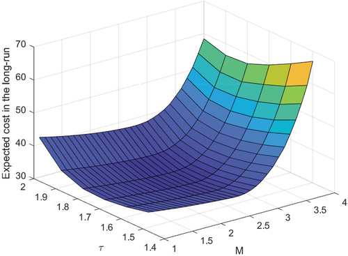
Figure 4 shows the variation of the expected cost rate in the long-run horizon with respect to the inspection interval with different settings of the failure threshold $L$ and the preventive maintenance threshold $M$.

Figure 4. The variation of the expected cost rate in the long-run horizon with respect to the inspection interval $\tau$.

It is observed that the cost rate in the long run is smaller for the system with larger failure threshold $L$. This is due to the fact that the system reliability increases with the failure threshold $L$. Hence, less budget is needed to distribute to the manufacturing and maintenance process. Also, with a larger preventive maintenance threshold $M$, the cost is more significant due to the higher expected restoration cost of the nonconforming products and larger system failure probabilities during two consecutive inspection intervals. 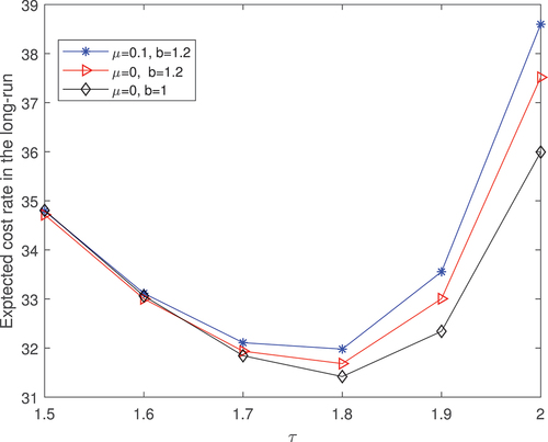Under each scenario, the expected cost rate during the manufacturing and maintenance process is a convex function of the inspection interval in the considered range, which implies the existence of the optimal lot-sizing ($Q=p\tau$) for a given deterministic production rate in this case. Figure 5 illustrates the influence of the dependence effect between $X_t^{(1)}$, $X_t^{(2)}$ and the out-of-control rate on the expected manufacturing and maintenance cost rate in the infinite horizon. Compared with the independence of the in-control/out-of-control state and the machine deterioration process ($\mu =0$), the dependence induces negative effect on the cost budget, which indicates that it is necessary to consider the interactions between the indicators of the system state in evaluating the manufacturing and maintenance budget. Whenever the sojourn time in the in-control state degenerates to the exponential distribution, as illustrated in the diamond line, the cost induced in the manufacturing and maintenance process is smaller due to the lower shift to the out-of-control state of the equipment.

Figure 5. The expected cost rate in the long-run horizon with different $\mu$ and $b$.

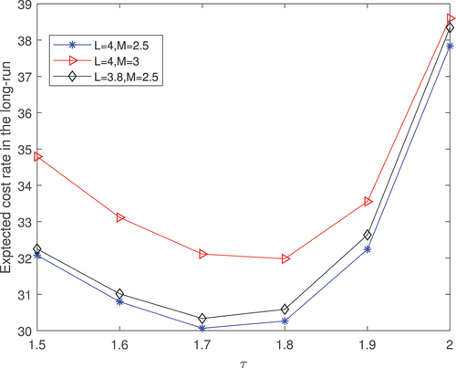
Figures 6–7 further illustrate the optimal expected cost rate in the long run under the above two situations. Both the optimum achieves at ${\tau }^{\ast }=1.7,M^{\ast }=2.6$, which indicates that the optimal lot-sizing is 34 and the optimal preventive maintenance threshold is 2.6, a little higher than $M_s$, the boundary between the two defective item rates. $C_{\mathrm{\infty }}(Q^{\ast },M^{\ast })$ arrives at 30.0496 and 29.2905, respectively, in the above scenarios.

Figure 6. The expected cost rate in the long-run horizon with different $\tau$ and $M$ given $\mu =0.1$.

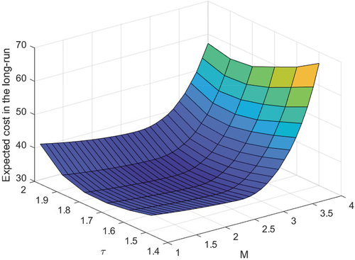
Figure 7. The expected cost rate in the long-run horizon with different $\tau$ and $M$ given $\mu =0$.

Table 4 summarizes the optimal $C_{\mathrm{\infty }}(Q^{\ast },M^{\ast })$ with respect to various parameter settings of the system with the rest of the parameters remain unchanged as illustrated in Table 4. Some phenomena can be observed from the table. It can be observed that with a larger demand requirement, the cost induced in the manufacturing and maintenance process is larger. With a larger $d$, the consumption of the product is quicker, while the transition time between two consecutive system states is smaller. Thus, the mean cycle is shorter. For instance, considering the scenario that no maintenance action is executed, the transition period decreases from $2\tau$ to $\frac{7}{4}\tau$. Meanwhile, the increase in the holding cost is not that significant. Thus, the cost rate decreases. We can also observe that the item defective rate may impact the optimal lot-size and the optimum cost. With a larger defective rate when the degradation level is below the threshold $M_s$, the optimum cost becomes larger and the optimal lot size gets smaller. When the degradation level is beyond $M_s$, similarly, the lot-size becomes larger with a little milder defect rate. It seems that to optimize the cost induced in the manufacturing and maintenance process, the manufacturer intends to expand the production by choosing a larger production run with a lower product defective rate. In addition, by varying the failure threshold and the defective rate threshold, the corresponding optimal policies are also presented. We can find the variation of the optimal preventive maintenance threshold. For the system with a lower failure threshold, the optimal preventive maintenance threshold is lower and the optimum cost is higher due to the shorter expected lifetime of the machine. Also, the variation of the optimum cost with respect to the maintenance cost unit and the maintenance time is also illustrated. The cost increases with the corrective maintenance cost $c_f$. It decreases with the maintenance time $t_f$, as the same maintenance cost is shared in a longer period.

Table 4. $C_{\mathrm{\infty }}(Q^{\ast },M^{\ast })$in the long run with various parameter settings.

Parameter settings
$d$	$r_0$	$r_1$	$L$	$M_s$	$t_f$	$c_f$	Optimum cost	Optimum $(Q^{\ast },M^{\ast })$
10	0.02	0.1	4	2.5	1	500	30.0496	(34, 2.6)
12	0.02	0.1	4	2.5	1	500	37.1434	(34, 2.6)
10	0.03	0.1	4	2.5	1	500	31.8492	(32, 2.6)
10	0.02	0.09	4	2.5	1	500	28.7408	(36, 2.6)
10	0.02	0.1	3.8	2.5	1	500	30.3345	(34, 2.5)
10	0.02	0.1	4	2.4	1	500	29.9857	(34, 2.5)
10	0.02	0.1	4	2.5	2	500	29.9286	(34, 2.6)
10	0.02	0.1	4	2.5	1	510	30.0952	(34, 2.6)

5. Conclusions

In this study, we have developed an integrated model that combines EMQ and CBM issues. Two dependent indicators are employed to represent the system states. One is modelled by a general distribution representing the sojourn time that the manufacturing process stays in the in-control state. One signifies the system deterioration which is described by a Gamma process with continuous state space and monotonic characteristic. When the manufacturing process is out-of-control or the system fails, costs are induced due to the quality loss, shortage loss, etc. For the production manager, how to schedule the inspection period to verify the system state? When the system state information is available, how to schedule the maintenance planning to control its production budget? We assess the problem by the expected cost including the holding cost, quality loss, inspection and maintenance costs per unitary time in the infinite horizon. The optimum of lot-sizing and the preventive maintenance threshold is derived. It can provide reference for the decision-maker in developing effective and integrated production and maintenance strategies.

Some issues could be further addressed in the future. First, this study considers a machine consisting of a single component producing a single type of product. A machine with multiple components and various configurations can be further evaluated. Secondly, the production and demand rates are supposed to be constant in our work. Random or stochastic production and demand rate is an interesting and challenging subject which can be further studied. Thirdly, we have assumed perfect inspection in this model, where the indicator information can be obtained perfectly upon inspection. An interesting topic is the imperfect inspection or partially revealed system state, where managerial decisions are based on imperfect information. These problems will be addressed in our further work.

Disclosure statement

No potential conflict of interest was reported by the authors.

Data availability statement

Due to the nature of this research, no hidden data are there for sharing that support the results or analyses presented in this work. All data used for carrying this research work are already available in this manuscript.

Additional information

Funding

This work is supported by the National Natural Science Foundation of China (61827901,71901026)

References

- Abdur Rahim, M., & Ben Daya, M. (2012). Integrated models in production planning, inventory, quality, and maintenance. Springer Science & Business Media.
- Boukas, E.K., & Liu, Z.K. (2001). Production and maintenance control for manufacturing systems. IEEE Transactions on Automatic Control, 46(9), 1455–1460. https://doi.org/10.1109/9.948477
- Chakraborty, T., & Giri, B.C. (2012). Joint determination of optimal safety stocks and production policy for an imperfect production system. Applied Mathematical Modelling, 36(2), 712–722. https://doi.org/10.1016/j.apm.2011.07.012
- Chakraborty, T., & Giri, B.C. (2014). Lot sizing in a deteriorating production system under inspections, imperfect maintenance and reworks. Operational Research, 14(1), 29–50. https://doi.org/10.1007/s12351-013-0134-5
- Cheng, G.Q., Zhou, B.H., & Li, L. (2018). Integrated production, quality control and condition-based maintenance for imperfect production systems. Reliability Engineering & System Safety, 175, 251–264. https://doi.org/10.1016/j.ress.2018.03.025
- Glock, C. H. (2012). The joint economic lot size problem: A review. International Journal of Production Economics, 135(2), 671–686. https://doi.org/10.1016/j.ijpe.2011.10.026
- Glock, C. H., Grosse, E. H., & Ries, J. M. (2014). The lot sizing problem: A tertiary study. International Journal of Production Economics, 155, 39–51. https://doi.org/10.1016/j.ijpe.2013.12.009
- Hadidi, L. A., Al-Turki, U. M., & Rahim, A. (2012). Integrated models in production planning and scheduling, maintenance and quality: A review. International Journal of Industrial and Systems Engineering, 10(1), 21–50.
- Hong-Fwu, Y., & Chen, Y. (2018). An integrated inventory model for items with acceptable defective items under warranty and quality improvement investment. Quality Technology & Quantitative Management, 15(6), 702–715. https://doi.org/10.1080/16843703.2017.1335490
- Hu, J., & Chen, P. (2020). Predictive maintenance of systems subject to hard failure based on proportional hazards model. Reliability Engineering & System Safety, 196, 106707. https://doi.org/10.1016/j.ress.2019.106707
- Jafari, L., & Makis, V. (2015). Joint optimal lot sizing and preventive maintenance policy for a production facility subject to condition monitoring. International Journal of Production Economics, 169, 156–168. https://doi.org/10.1016/j.ijpe.2015.07.034
- Jafari, L., & Makis, V. (2016). Optimal lot-sizing and maintenance policy for a partially observable production system. Computers & Industrial Engineering, 93, 88–98. https://doi.org/10.1016/j.cie.2015.12.009
- Jafari, L., & Makis, V. (2019). Optimal production and maintenance policy for a partially observable production system with stochastic demand. International Journal of Industrial and Systems Engineering, 13(7), 449–456. https://doi.org/10.5281/zenodo.3300342
- Jiang, W., & Farr, J. V. (2007). Integrating SPC and EPC methods for quality improvement. Quality Technology & Quantitative Management, 4(3), 345–363. https://doi.org/10.1080/16843703.2007.11673156
- Malik, A., & Sarkar, B. (2020). Disruption management in a constrained multi-product imperfect production system. Journal of Manufacturing Systems, 56, 227–240. https://doi.org/10.1016/j.jmsy.2020.05.015
- Mercier, S., Meier-Hirmer, C., & Roussignol, M. (2012). Bivariate gamma wear processes for track geometry modelling, with application to intervention scheduling. Structure and Infrastructure Engineering, 8(4), 357–366. https://doi.org/10.1080/15732479.2011.563090
- Ouaret, S., Kenné, J.-P., & Gharbi, A. (2018). Production and replacement policies for a deteriorating manufacturing system under random demand and quality. European Journal of Operational Research, 264(2), 623–636. https://doi.org/10.1016/j.ejor.2017.06.062
- Park, M. (2021). Optimal production policy for economic production lot-sizing model with preventive maintenance. Quality Technology & Quantitative Management, 18(1), 83–100. https://doi.org/10.1080/16843703.2020.1766740
- Peng, H., & van Houtum, G.-J. (2016). Joint optimization of condition-based maintenance and production lot-sizing. European Journal of Operational Research, 253(1), 94–107. https://doi.org/10.1016/j.ejor.2016.02.027
- Polyanin, A. D., & Manzhirov, A. V. (2008). Handbook of integral equations. Chapman and Hall/CRC.
- Qiu, Q., Cui, L., & Shen, J. (2019). Availability analysis and maintenance modelling for inspected Markov systems with down time threshold. Quality Technology & Quantitative Management, 16(4), 478–495. https://doi.org/10.1080/16843703.2018.1465228
- Rosenblatt, M. J., & Lee, H. L. (1986). Economic production cycles with imperfect production processes. IIE Transactions, 18(1), 48–55. https://doi.org/10.1080/07408178608975329
- Sana, S., & Chaudhuri, K. (2010). An EMQ model in an imperfect production process. International Journal of Systems Science, 41(6), 635–646. https://doi.org/10.1080/00207720903144495
- Sana, S.S., Goyal, S.K., & Chaudhuri, K. (2007). An imperfect production process in a volume flexible inventory model. International Journal of Production Economics, 105(2), 548–559. https://doi.org/10.1016/j.ijpe.2006.05.005
- Sarkar, B., Mandal, P., & Sarkar, S. (2014). An EMQ model with price and time dependent demand under the effect of reliability and inflation. Applied Mathematics and Computation, 231, 414–421. https://doi.org/10.1016/j.amc.2014.01.004
- Sarkar, B., Sankar Sana, S., & Chaudhuri, K. (2010). Optimal reliability, production lotsize and safety stock: An economic manufacturing quantity model. International Journal of Management Science and Engineering Management, 5(3), 192–202.
- Scarf, P.A. (2007). A framework for condition monitoring and condition based maintenance. Quality Technology & Quantitative Management, 4(2), 301–312. https://doi.org/10.1080/16843703.2007.11673152
- Sicilia, J., González De la Rosa, M., Febles-Acosta, J., & Alcaide López de Pablo, D. (2014). Optimal policy for an inventory system with power demand, backlogged shortages and production rate proportional to demand rate. International Journal of Production Economics, 155, 163–171. https://doi.org/10.1016/j.ijpe.2013.11.020
- Sloan, T. W., & Shanthikumar, G.J. (2000). Combined production and maintenance scheduling for a multiple-product, single-machine production system. Production and Operations Management, 9(4), 379–399. https://doi.org/10.1111/j.1937-5956.2000.tb00465.x
- Wang, L., Yang, Y., Zhu, H., & Liu, G. (2020). Optimal condition-based renewable warranty policy for products with three-stage failure process. Quality Technology & Quantitative Management, 17(2), 216–233. https://doi.org/10.1080/16843703.2019.1584956
- Zhang, Y. (2018). Condition-based maintenance models: Application to subsea safety systems.
- Zhang, N., Fouladirad, M., Barros, A., & Zhang, J. (2020). Condition-based maintenance for a k-out-of-n deteriorating system under periodic inspection with failure dependence. European Journal of Operational Research, 287(1), 159–167. https://doi.org/10.1016/j.ejor.2020.04.041
- Zhang, F., Shen, J., & Ma, Y. (2020). Optimal maintenance policy considering imperfect repairs and non-constant probabilities of inspection errors. Reliability Engineering & System Safety, 193, 106615. https://doi.org/10.1016/j.ress.2019.106615
- Zheng, R., & Zhou, Y. (2022). A dynamic inspection and replacement policy for a two-unit production system subject to interdependence. Applied Mathematical Modelling, 103, 221–237. https://doi.org/10.1016/j.apm.2021.10.028
- Zheng, R., Zhou, Y., Gu, L., & Zhang, Z. (2021). Joint optimization of lot sizing and condition-based maintenance for a production system using the proportional hazards model. Computers & Industrial Engineering, 154, 107157. https://doi.org/10.1016/j.cie.2021.107157