Bayesian benefits with JASP

Abstract

We illustrate the Bayesian approach to data analysis using the newly developed statistical software program JASP. With JASP, researchers are able to take advantage of the benefits that the Bayesian framework has to offer in terms of parameter estimation and hypothesis testing. The Bayesian advantages are discussed using real data on the relation between Quality of Life and Executive Functioning in children with Autism Spectrum Disorder.

Keywords:

• Correlation test
• credible interval
• Bayes factor
• JASP

In recent years it has become increasingly apparent that the Bayesian approach to data analysis comes with considerable advantages, both theoretically and practically (e.g. Dienes, 2008, 2011; Gelman et al., 2014; Gill, 2015; Hoijtink, Klugkist, & Boelen, 2008; Kruschke, 2010; Lee & Wagenmakers, 2013; Mulder & Wagenmakers, 2016; Wagenmakers, 2007; Wagenmakers, Morey, & Lee, 2016; for a systematic overview of more than 1500 articles reporting Bayesian analyses in psychology see van der Schoot, Winter, Ryan, Zondervan-Zwijnenburg, & Depaoli, in press). For example, researchers who use Bayesian statistics can express their confidence for a parameter being in any particular range (e.g. Morey, Hoekstra, Rouder, Lee, & Wagenmakers, 2016; Pratt, 1961); they can express the evidence for or against hypotheses on a continuous scale (e.g. Jeffreys, 1961; Kass & Raftery, 1995); finally, they can monitor the evidential trajectory in real time, as the data accumulate (e.g. Anscombe, 1963; Berger & Wolpert, 1988; Rouder, 2014; Schönbrodt, Wagenmakers, Zehetleitner, & Perugini, in press). In sum, the Bayesian statistical paradigm unlocks advantages that remain out of reach for researchers who continue to use only frequentist statistics (e.g. reporting p values for hypothesis testing and reporting confidence intervals for parameter estimation).

However, one major obstacle prevents pragmatic researchers from taking full advantage of the possibilities that the Bayesian framework has to offer: for most researchers it takes a prohibitive investment of effort, time and patience to derive and programme even the most basic Bayesian analysis. Thus, an important impediment to the widespread use of the Bayesian approach to data analysis is the lack of easy-to-use software that support Bayesian methods for common statistical tests.

To overcome this obstacle, we have recently developed the free and open-source statistical software program JASP (JASP Team, 2016; jasp-stats.org). JASP features both classical and Bayesian implementations of the most popular tests in psychological research, that is, t-tests, ANOVAs, correlation tests, linear regression and tests for contingency tables. Importantly, JASP is intuitive and comes with a simple and attractive graphical user interface shown in Figure 1. JASP includes the ability to annotate analyses, to share data and analyses on the Open Science Framework (osf.io), to copy-paste APA-formatted tables into popular text editors such as Microsoft Word, and to generate informative and publication-ready figures.

Figure 1. A screenshot of JASPs graphical user interface; analysis input options can be set in the left panel and dynamically adjusted output is displayed in the right panel.

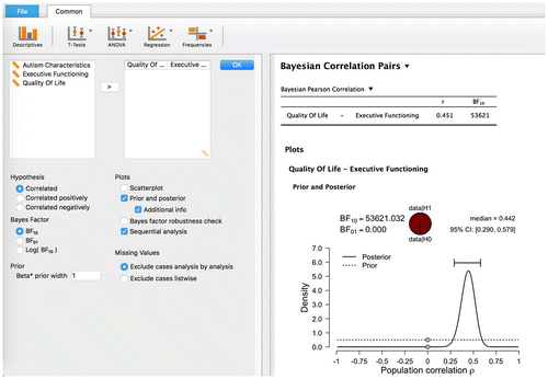
In this article, we use a real-data example of a correlation analysis to showcase JASP and some of the advantages that a Bayesian analysis has to offer. Specifically, we will demonstrate how to use JASP for Bayesian parameter estimation, Bayesian hypothesis testing and Bayesian sequential analyses. An annotated .jasp-file is available at the Open Science Framework (osf.io/m2quv), which can be viewed without having JASP installed.

Example: Quality of Life and Executive Functioning for children with ASD

Throughout this article we use data from de Vries and Geurts (2015) to illustrate several Bayesian analyses implemented in JASP. De Vries and Geurts studied the relation between Quality of Life (QoL) and Executive Functioning (EF) in children with and without Autism Spectrum Disorder (ASD). We focus on a subset of their data and analyze the correlation between QoL and EF in n = 119 children with ASD. Both QoL and EF were assessed using standardized questionnaires (see Bastiaansen, Koot, Bongers, Varni, & Verhulst, 2004; de Vries & Geurts, 2015; Gioia, Isquith, Guy, & Kenworthy, 2000; Smidts & Huizinga, 2009; Varni, Seid, & Kurtin, 2001, for further details).

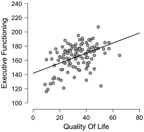
Figure 2 shows a scatterplot of the QoL and EF scores for the children with ASD. The observed Pearson correlation coefficient is r = .451, and a classical analysis reveals that the correlation is significant (p < .001), suggesting that the null hypothesis H₀ : ρ = 0 can be rejected. Below we showcase three different Bayesian analyses from JASP that arguably provide a more complete statistical assessment.

Figure 2. A scatterplot of scores on the PedsQL-questionnaire measuring QoL and on the BRIEF-questionnaire measuring EF for n = 119 children with ASD.

Analysis I: Bayesian parameter estimation

In our first analysis we wish to use the observed data to update our knowledge about the latent correlation ρ. The possibility that ρ = 0 is not of special interest – our goal is to estimate the size of the correlation, not to test whether the correlation is present or absent. In order that the data may be used to update our knowledge about ρ we need to specify our knowledge about ρ before any data are observed. Bayesians do this by specifying a prior distribution which expresses advance knowledge, uncertainty, belief, or the relative plausibility of the possible values for ρ. Here we specify a prior distribution which asserts that every value of ρ between −1 and +1 is equally plausible a priori (Jeffreys, 1961). This uniform specification is the default option in JASP.

The prior distribution is updated using the information in the data to yield a posterior distribution. The posterior distribution expresses our uncertainty about the unknown ρ after having seen the data. Figure 3 shows the prior distribution and the posterior distribution for ρ obtained after updating using the example data from the ASD children. Figure 3 reveals that the posterior distribution for ρ is more peaked than the prior distribution, which indicates that we have learned about ρ from the observed data.

Figure 3. JASP graphical output for the Bayesian correlation analysis.

Notes: The prior distribution for the correlation coefficient ρ is indicated by a dashed line, and the posterior distribution is indicated by a solid line. Also displayed are the posterior median, the central 95% credible interval, and the Bayes factors BF₁₀ and BF₀₁.

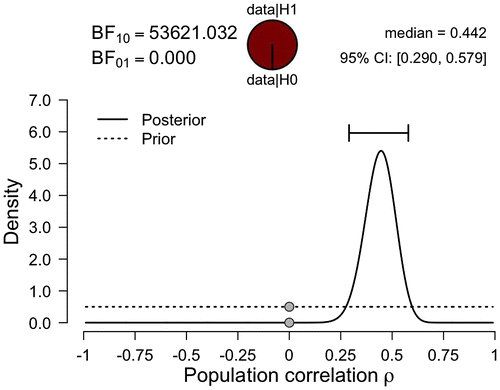
When we compare the prior distribution to the posterior distribution, we see that the prior distribution assigns considerable plausibility to values lower than .20 and values higher than .70, 75% to be exact, whereas the posterior distribution assigns only little plausibility to these values. Furthermore, the central 95% credible interval ranges from .29 to about .58, which implies that we can be 95% confident that the true value of ρ lies between .29 and .58. Note that such an intuitive statement cannot be obtained within the classical statistical framework (e.g. Berger & Wolpert, 1988; Morey, Hoekstra, Rouder, & Wagenmakers, 2016; Morey et al., 2016; Pratt, 1961). Finally, it should be stressed that Figure 3 is obtained in JASP by simply dragging and dropping the relevant variables in the graphical user interface. No programming or mathematical derivation is required.¹

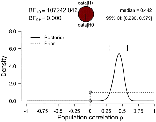
A characteristic advantage that the Bayesian approach has to offer is the ability to incorporate prior information. For instance, previous results and theory described by de Vries and Geurts (2015) anticipated a positive correlation between QoL and EF for children with ASD, suggesting the one-sided hypothesis H₊ : ρ > 0. This information can be incorporated by updating the prior distribution through the order constraint ρ ≥ 0, such that we assume that each value of ρ between 0 and 1 is equally plausible a priori (Hoijtink, 2011; Hoijtink et al., 2008; Klugkist, Laudy, & Hoijtink, 2005). The addition of this order restriction requires setting a single tick mark in the JASP input panel.

The results based on this new prior distribution are shown in Figure 4. Since the prior distribution needs to integrate to unity (i.e. the area under the curve equals 1), we observe that the prior density in Figure 4 is twice as high as the prior density in Figure 3. A comparison of the posterior distributions in Figures 3 and 4 reveals that the order restriction did not alter the posterior distribution in a meaningful way. The reason for this robustness is that most of the posterior mass was already consistent with the restriction.

Figure 4. JASP graphical output for the Bayesian correlation analysis incorporating the prior information that ρ > 0.

Notes: The prior distribution for the correlation coefficient ρ is indicated by a dashed line, and the posterior distribution is indicated by a solid line. Also displayed are the posterior median, the central 95% credible interval, and the Bayes factors BF₊₀ and BF₀₊.

Analysis II: Bayesian hypothesis testing

As mentioned earlier, the Bayesian parameter estimation approach presupposes that the correlation is relevant, that is, that ρ ≠ 0, but we have not seriously considered the situation that the correlation is irrelevant, that is, that ρ = 0.

If the goal is hypothesis testing, we need to assess the predictive adequacy of the null hypothesis H₀ : ρ = 0 that stipulates the correlation to be absent, and contrast this against the predictive adequacy of an alternative hypothesis H₁ that stipulates the correlation to exist (Wagenmakers et al., 2016). Without explicitly taking H₀ into consideration, it is not possible to make meaningful statements about the presence or absence of an effect (e.g. Wrinch & Jeffreys, 1921).

In order to compare the predictive adequacy of H₀ against H₁, the hypotheses have to be translated to statistical models, which requires the specification of prior distributions for ρ under each of the hypotheses. Under H₀, the prior on ρ is a point mass at zero (but see Morey & Rouder, 2011 for an alternative specification); under H₁, ρ is assigned a prior distribution that relaxes the restriction-to-zero. Here we employ the default uniform prior distributions that we also used to estimate the parameters in Figures 3 and 4.

With the models relating to H₀ and H₁ fully specified, we may compare their relative predictive performance using the Bayes factor (Jeffreys, 1961):

The subscripts ‘10’ in BF₁₀ indicate that the model associated with H₁ is in the numerator and that the model associated with H₀ is in the denominator. That is, BF₁₀ = 1/BF₀₁. Similarly, we use BF₊₀ to express the comparison of H₊ to H₀. When the Bayes factor BF₁₀ equals 20, the data are 20 times more likely under H₁ than under H₀. Similarly, when the Bayes factor BF₁₀ is equal to .05, the data are 20 times more likely under H₀ than under H₁.

The Bayes factors for our example are shown in the top part of Figures 3 and 4, and reveal overwhelming evidence against H₀. Specifically, the Bayes factor BF₁₀ shown in Figure 3 indicates that the observed data are over 50,000 times more likely under H₁ (i.e. the unconstrained hypothesis that the correlation is either positive or negative) than under H₀. Similarly, the Bayes factor BF₊₀ (i.e. the constrained hypothesis that the correlation is positive-only) shown in Figure 4 indicates that the observed data are over 100,000 times more likely under H₊ than under H₀. Both Bayes factors indicate that the observed data provide overwhelming support for the existence of a positive correlation between QoL and EF for children with ASD. Note that in classical statistics the nature of the support in favour of the alternative hypothesis is much less direct: the p-value is based on what can be expected if the null hypothesis were true, and ignores what can be expected if the alternative hypothesis were true (e.g. Berkson, 1938).

Given that the posterior distributions shown in Figures 3 and 4 are located away from ρ = 0 it should not come as a surprise that the evidence against H₀ is overwhelming. However, it may come as a surprise that the evidence is almost twice as strong in favour of H₊ than it is in favour of H₁; after all, the posterior distributions for ρ are virtually identical under both hypotheses.

Both regularities can be clarified using the Savage–Dickey density ratio method, a useful shortcut that allows the Bayes factor to be easily computed and visualized (Dickey & Lientz, 1970; Wagenmakers, Lodewyckx, Kuriyal, & Grasman, 2010). Assume we wish to compare a point hypothesis H₀ (e.g. ρ = 0) to an encompassing alternative H₁ (e.g. ρ ~ Uniform (−1, 1)). Then the Savage–Dickey identity holds that the Bayes factor BF₁₀ can be obtained from a consideration of the prior and posterior distribution under H₁. Specifically, the Bayes factor BF₁₀ is given by the ratio of the height of the posterior distribution for ρ evaluated at ρ = 0 against the height of the prior distribution for ρ evaluated at ρ = 0. These points are shown as the gray dots in Figures 3 and 4.

The intuitive result that posteriors away from zero correspond to overwhelming evidence against H₀ follows from the Savage–Dickey identity – when the posterior is away from zero, the height of the prior at ρ = 0 will be much higher than the height of the posterior at ρ = 0.

The counter-intuitive result that the evidence is almost twice as strong in favour of H₊ than it is in favour of H₁ also follows from the Savage–Dickey identity – whereas the posterior distributions of ρ under H₁ and H₊ hardly differ, the prior density at ρ = 0 for H₊ is twice as high as the prior density at ρ = 0 for H₁. Conceptually, the restricted hypothesis makes more specific and daring predictions than H₁, which hedges its bets and distributes its predictions more widely. When the data are consistent with the restriction, the more daring hypothesis should be rewarded, receiving a bonus for parsimony (e.g. Jefferys & Berger, 1992; Klugkist, van Wesel, & Bullens, 2011; Lee & Wagenmakers, 2013, Chapter 7; Myung & Pitt, 1997; Vanpaemel, 2010). The prior distribution directly affects the model predictions (i.e. model parsimony), and consequently the prior distribution also directly affects the Bayes factor. Therefore, Bayes factor hypothesis testing requires that prior distributions are selected with special care. Fortunately, much development in ‘objective Bayesian statistics’ has concerned the construction of prior distributions that obey a series of desiderata, such that these priors are suitable for a reference-style analysis that may be refined when additional information is available (e.g. Bayarri, Berger, Forte, & García-Donato, 2012; for a discussion see Wagenmakers et al., 2016).

Analysis III: Bayesian sequential analysis

Another practical advantage of the Bayesian approach to data analysis is that researchers are free to monitor the evidence as the data accumulate, for example in the form of a Bayes factor or a posterior distribution (e.g. Berger & Berry, 1988; Edwards, Lindman, & Savage, 1963; Kadane, Schervish, & Seidenfeld, 1996; Rouder, 2014; Schönbrodt et al., in press; Wagenmakers, Wetzels, Borsboom, van der Maas, & Kievit, 2012; Wagenmakers et al., 2016). As summarized by Anscombe (1963, p. 381),

So long as all observations are fairly reported, the sequential stopping rule that may or may not have been followed is irrelevant. The experimenter should feel entirely uninhibited about continuing or discontinuing his trial, changing his mind about the stopping rule in the middle, etc., because the interpretation of the observations will be based on what was observed, and not on what might have been observed but wasn’t.

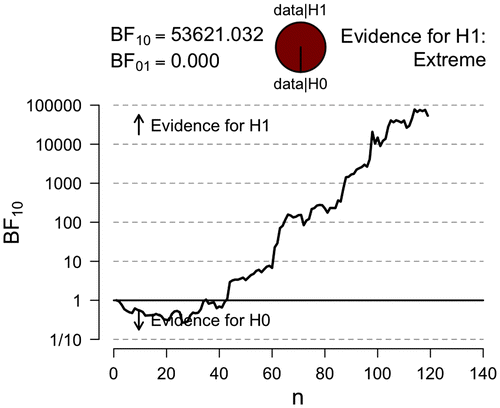
In other words, a researcher using Bayesian statistics may terminate data collection when the evidence is overwhelming and further data collection would be a waste of time, energy and money. Similarly, that researcher may decide to collect additional observations in case the interim results are not sufficiently compelling. This flexibility in data collection releases researchers from the straitjacket imposed by classical statistics (e.g. Armitage, McPherson, & Rowe, 1969; Feller, 1940, 1970) and makes for experimentation that is both efficient and ethical. In JASP, a graph of the evidential trajectory can be obtained by setting a single tick mark.

Figure 5 illustrates the evidential trajectory in favour of H₁ over H₀ and shows that the evidence (shown on the y-axis) increases with the number of data points (shown on the x-axis). From Figure 5 we observe that after about 60 observations the Bayes factor equals 10 and after about 90 observations the Bayes factor equals 1000. Note that initially, for small values of n, the Bayes factor indicates modest evidence for H₀; in other words, when little information is available the Bayes factor prefers the more parsimonious model, as is desirable.

Figure 5. JASP graphical output for the sequential analysis that displays the flow of evidence for H₁ : ρ ~ Uniform (−1, 1) vs. H₀: ρ = 0 as the data accumulate.

Note: The sequence of data points n is shown on the x-axis and the associated Bayes factor is shown on the y-axis.

Concluding comments

Using data on QoL and EF in ASD children we showed how JASP can be exploited to obtain a series of informative Bayesian results. Specifically, we indicated how researchers can adopt the Bayesian framework to estimate an unknown correlation, to test for the presence of the correlation, and to monitor the evidential flow as the data accumulate. Whether viewed as an alternative or as a wholesale replacement of classical inference procedures, the Bayesian approach provides distinctive benefits and encourages a flexible and intelligent approach to data analysis. Armed with JASP, these Bayesian benefits are only a mouse click away.

Disclosure statement

No potential conflict of interest was reported by the authors.

Funding

This work was supported by the European Research Council [grant number 283876].

Notes

1 For an indication of the mathematics that have been derived ‘behind the scenes’ see http://arxiv.org/ abs/1510.01188.

References

- Anscombe, F. J. (1963). Sequential medical trials. Journal of the American Statistical Association, 58, 365–383.10.1080/01621459.1963.10500851
- Armitage, P., McPherson, C. K., & Rowe, B. C. (1969). Repeated significance tests on accumulating data. Journal of the Royal Statistical Society. Series A (General), 132, 235–244.10.2307/2343787
- Bastiaansen, D., Koot, H., Bongers, I., Varni, J., & Verhulst, F. (2004). Measuring quality of life in children referred for psychiatric problems: Psychometric properties of the PedsQLTM 4.0 generic core scales. Quality of Life Research, 13, 489–495.10.1023/B:QURE.0000018483.01526.ab
- Bayarri, M. J., Berger, J. O., Forte, A., & García-Donato, G. (2012). Criteria for Bayesian model choice with application to variable selection. The Annals of Statistics, 40, 1550–1577.10.1214/12-AOS1013
- Berger, J. O., & Berry, D. A. (1988). The relevance of stopping rules in statistical inference. In S. S. Gupta & J. O. Berger (Eds.), Statistical decision theory and related topics (Vol. 1, pp. 29–48). New York, NY: Springer Verlag.10.1007/978-1-4613-8768-8
- Berger, J. O., & Wolpert, R. L. (1988). The likelihood principle (2nd ed.). Hayward, CA: Institute of Mathematical Statistics.
- Berkson, J. (1938). Some difficulties of interpretation encountered in the application of the chi-square test. Journal of the American Statistical Association, 33, 526–536.10.1080/01621459.1938.10502329
- de Vries, M., & Geurts, H. (2015). Influence of autism traits and executive functioning on quality of life in children with an autism spectrum disorder. Journal of Autism and Developmental Disorders, 45, 2734–2743.10.1007/s10803-015-2438-1
- Dickey, J. M., & Lientz, B. P. (1970). The weighted likelihood ratio, sharp hypotheses about chances, the order of a Markov chain. The Annals of Mathematical Statistics, 41, 214–226.10.1214/aoms/1177697203
- Dienes, Z. (2008). Understanding psychology as a science: An introduction to scientific and statistical inference. New York, NY: Palgrave MacMillan.
- Dienes, Z. (2011). Bayesian versus orthodox statistics: Which side are you on? Perspectives on Psychological Science, 6, 274–290.10.1177/1745691611406920
- Edwards, W., Lindman, H., & Savage, L. J. (1963). Bayesian statistical inference for psychological research. Psychological Review, 70, 193–242.10.1037/h0044139
- Feller, W. (1940). Statistical aspects of ESP. Journal of Parapsychology, 4, 271–298.
- Feller, W. (1970). An introduction to probability theory and its applications (Vol. I). New York, NY: Wiley.
- Gelman, A., Carlin, J. B., Stern, H. S., Dunson, D. B., Vehtari, A., & Rubin, D. B. (2014). Bayesian data analysis (3rd ed.). Boca Raton, FL: Chapman & Hall/CRC.
- Gill, J. (2015). Bayesian methods: A social and behavioral sciences approach (3rd ed.). Boca Raton, FL: CRC Press.
- Gioia, G., Isquith, P., Guy, S., & Kenworthy, L. (2000). TEST REVIEW behavior rating inventory of executive functioning. Child Neuropsychology, 6, 235–238.10.1076/chin.6.3.235.3152
- Hoijtink, H. (2011). Informative hypotheses: Theory and practice for behavioral and social scientists. Boca Raton, FL: Chapman & Hall/CRC.10.1201/CHSTSOBESCI
- Hoijtink, H., Klugkist, I., & Boelen, P. (2008). Bayesian evaluation of informative hypotheses. New York, NY: Springer.10.1007/978-0-387-09612-4
- JASP Team. (2016). JASP (Version 0.7.5.6) [Computer software]. Retrieved from https://jasp-stats.org/
- Jefferys, W. H., & Berger, J. O. (1992). Ockham’s razor and Bayesian analysis. American Scientist, 80, 64–72.
- Jeffreys, H. (1961). Theory of probability (3rd ed.). Oxford: Oxford University Press.
- Kadane, J. B., Schervish, M. J., & Seidenfeld, T. (1996). Reasoning to a foregone conclusion. Journal of the American Statistical Association, 91, 1228–1235.10.1080/01621459.1996.10476992
- Kass, R. E., & Raftery, A. E. (1995). Bayes factors. Journal of the American Statistical Association, 90, 773–795.10.1080/01621459.1995.10476572
- Klugkist, I., Laudy, O., & Hoijtink, H. (2005). Inequality constrained analysis of variance: A Bayesian approach. Psychological Methods, 10, 477–493.10.1037/1082-989X.10.4.477
- Klugkist, I., van Wesel, F., & Bullens, J. (2011). Do we know what we test and do we test what we want to know? International Journal of Behavioral Development, 35, 550–560.10.1177/0165025411425873
- Kruschke, J. K. (2010). Doing Bayesian data analysis: A tutorial introduction with R and BUGS. Burlington, MA: Academic Press.
- Lee, M. D., & Wagenmakers, E.-J. (2013). Bayesian modeling for cognitive science: A practical course. Cambridge: Cambridge University Press.10.1017/CBO9781139087759
- Morey, R. D., & Rouder, J. N. (2011). Bayes factor approaches for testing interval null hypotheses. Psychological Methods, 16, 406–419.10.1037/a0024377
- Morey, R. D., Hoekstra, R., Rouder, J. N., Lee, M. D., & Wagenmakers, E.-J. (2016). The fallacy of placing confidence in confidence intervals. Psychonomic Bulletin & Review, 23, 103–123.10.3758/s13423-015-0947-8
- Morey, R. D., Hoekstra, R., Rouder, J. N., & Wagenmakers, E.-J. (2016). Continued misinterpretation of confidence intervals: Response to Miller and Ulrich. Psychonomic Bulletin & Review, 23, 131–140.10.3758/s13423-015-0955-8
- Mulder, J., & Wagenmakers, E.-J. (2016). Editor’s introduction to the special issue on “Bayes factors for testing hypotheses in psychological research: Practical relevance and new developments”. Journal of Mathematical Psychology, 72, 1–5.10.1016/j.jmp.2016.01.002
- Myung, I. J., & Pitt, M. A. (1997). Applying Occam’s razor in modeling cognition: A Bayesian approach. Psychonomic Bulletin & Review, 4, 79–95.10.3758/BF03210778
- Pratt, J. W. (1961). Review of Lehmann, E. L., testing statistical hypotheses. Journal of the American Statistical Association, 56, 163–167.10.2307/2282344
- Rouder, J. N. (2014). Optional stopping: No problem for Bayesians. Psychonomic Bulletin & Review, 21, 301–308.10.3758/s13423-014-0595-4
- Schönbrodt, F. D., Wagenmakers, E.-J., Zehetleitner, M., & Perugini, M. (in press). Sequential hypothesis testing with Bayes factors: Efficiently testing mean differences. Psychological Methods.
- Smidts, D., & Huizinga, M. (2009). BRIEF executive functies vragenlijst: Handleiding. Amsterdam: Hogrefe Uitgevers.
- van der Schoot, R., Winter, S., Ryan, O., Zondervan-Zwijnenburg, M., & Depaoli, S. (in press). A systematic review of Bayesian papers in psychology: The last 25 years. Psychological Methods.
- Vanpaemel, W. (2010). Prior sensitivity in theory testing: An apologia for the Bayes factor. Journal of Mathematical Psychology, 54, 491–498.10.1016/j.jmp.2010.07.003
- Varni, J., Seid, M., & Kurtin, P. (2001). PedsQL™ 4.0: Reliability and Validity of the Pediatric Quality of Life Inventory™ Version 4.0 Generic Core Scales in Healthy and Patient Populations. Medical Care, 39, 800–812.10.1097/00005650-200108000-00006
- Wagenmakers, E.-J. (2007). A practical solution to the pervasive problems of p values. Psychonomic Bulletin & Review, 14, 779–804.10.3758/BF03194105
- Wagenmakers, E.-J., Lodewyckx, T., Kuriyal, H., & Grasman, R. (2010). Bayesian hypothesis testing for psychologists: A tutorial on the Savage–Dickey method. Cognitive Psychology, 60, 158–189.10.1016/j.cogpsych.2009.12.001
- Wagenmakers, E.-J., Marsman, M., Jamil, T., Ly, A., Verhagen, A. J., Love, J., … Morey, R. D. (2016). Bayesian statistical inference for psychological science. Part I: Theoretical advantages and practical ramifications. Accepted pending minor revision, Psychonomic Bulletin & Review.
- Wagenmakers, E.-J., Morey, R. D., & Lee, M. D. (2016). Bayesian benefits for the pragmatic researcher. Current Directions in Psychological Science, 25, 169–176.10.1177/0963721416643289
- Wagenmakers, E.-J., Wetzels, R., Borsboom, D., van der Maas, H. L. J., & Kievit, R. A. (2012). An agenda for purely confirmatory research. Perspectives on Psychological Science, 7, 627–633.
- Wrinch, D., & Jeffreys, H. (1921). On certain fundamental principles of scientific inquiry. Philosophical Magazine Series 6, 42, 369–390.10.1080/14786442108633773