Evaluating time-dependent heat fluxes using artificial neural networks

Abstract

The inverse heat conduction problem (IHCP) is still challenging. Here is presented a new application of recurrent neural networks to estimate the heat flux applied on one side of a structure from the knowledge of the temperature measured at the other side of the structure (standard one-dimensional conducting bar). In the first part of the article the direct problem is solved and a model is determined. The mathematical inversion of this model leading to unsatisfactory results, a second approach is given in the second part of the study: to directly determine a representation of the mapping between the temperatures and the heat fluxes. After showing that satisfactory results are obtained when noisy data are considered, a final validation is carried out by coupling the direct model and the inverse model. The results are promising and it can be considered that recurrent neural networks are helpful tools to approach the solution of an inverse heat conduction problem.

Keywords:

• IHCP
• Inverse
• Conduction
• Heat
• Neural networks
• 2000 Mathematics Subject Classifications: 35K05
• 80A23
• 62M45

1. Introduction

It is necessary to solve an inverse heat conduction problem (IHCP) when it is not possible to introduce sensors where the interesting data should be measured, or when the boundary is not fixed as it is encountered in industrial furnaces 1. Such engineering applications of IHCP have led researchers to tackle the problem using different techniques. The sequential function method is largely used in its original form (e.g. 2–4), or with adaptations 5–7. Even the most recent developments led to oscillations from the retrieved data (fig. 6c page 2676 in 4). Recursive methods have also been used 8–10, but the solution is not totally satisfactory for sharp variations (fig. 4d page 279 in 10). The conjugate gradient method (e.g. 11–13) is also popular but its main drawback is its computational cost.

In 1999, Krejsa et al. 14 gave an assessment of strategies and potential for neural networks in the IHCP (see also 15). In 2002, Shiguemori et al. 16 compared the results obtained by the regularization method and results obtained using neural networks. They concluded that for a similar accuracy, the artificial neural networks are much faster. The networks used by these authors were traditional networks such as Back-Propagation or Radial Basis Functions networks. Although these kinds of networks can be successfully used to solve IHCP 17,18, it becomes difficult to use them when addressing time-dependent problems. To solve this kind of problems, and continue using artificial neural networks, it is necessary to move to recurrent networks 19. Some of them have recently been developed for online identification 20 and used in thermal engineering (e.g. 21,22). The aim of the present work is to show that, when they are well-tuned and well-trained, these neural networks can be successfully used to approach the solution of a time-dependent IHCP, as done for inverse problems in other fields 23,24. Although nonlinear problems can be addressed with these networks, only linear structures are studied here to make possible a comparison with already published data.

2. Description of the studied problem and calculation procedures

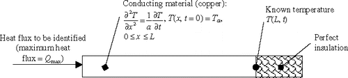
To evaluate the efficiency of a method, the authors study standard configurations, using standard excitations. The standard geometry mostly used in inverse heat conduction studies is the one-dimensional bar. As it has been shown that the quality of the method depends on the size of the bar 9, it has been chosen here to study one structure (figure 1) which leads to the largest discrepancies.

Figure 1. Schematic of the studied structure.

The following nondimensional quantities are defined:

-	heat flux: Q/Qmax,
-	temperature: T(x, t) − Ta/(Tmax(x = L) − Ta), the maximum temperature being defined for all the datasets used in the present study.

Two approaches are presented hereafter: the inversion of a direct model, and the direct determination of an inverse model. In any case, to get representative data, the direct problem (to compute the temperature at the insulated side from the knowledge of the heat flux) is solved numerically using a finite different scheme.

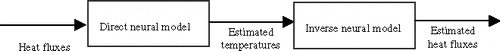
For the first approach, a model is determined that correctly predicts the temperatures from the knowledge of the heat fluxes. This model will later be referred to as the DM model (direct model). Its transfer function is mathematically inversed, so that a first “inverse model” is obtained (figure 2a). This model is referred to as the MIDM (Mathematical Inverse of the Direct Model) model.

Figure 2. Calculation procedures (a) inversing the direct model and (b) finding an inverse model.

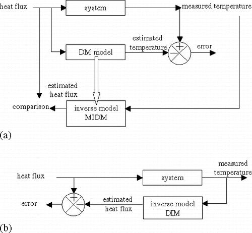
In the second approach, it is really the inverse problem (to compute the heat flux from the knowledge of the temperature at the insulated side) which is tackled. This is done through the inversion of the outputs and the inputs (figure 2b). The model that is obtained is the DIM (Direct Inverse Model) model.

For both approaches, a final validation is carried out coupling the “direct model” and the “inverse model”. Note that all the models are neural models obtained using recurrent neural networks. Each approach is detailed in a separate section.

3. The direct model and its inversion

The aim of this part is to find an acceptable representation of the relationship between the input data (the heat fluxes) and the output data (the temperatures). To do so, and as done whenever possible 25, a random sequence of input data is generated that leads to the knowledge of output data, and the identification process is carried out. The results are presented with a time step of 0.01 s, a thermal diffusivity a = 234.10⁻⁷ m²/s and a length L = 0.002 m, so the results are comparable with the results presented in 9. In this configuration, and knowing that the time step used for the calculations is 0.0001 s, the dimensionless time step, based on the length of the bar, is 5.84 × 10⁻⁴.

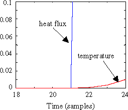
Figure 3 shows an example of the response of the structure for random heat fluxes. A detailed view of the response (figure 4) clearly shows the time lag (here one time step) that exists between the heat flux and the temperature at the other end of the bar.

Figure 3. Example of the response of the structure (direct problem).

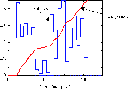
Figure 4. Detailed view of the response.

Many identification techniques could have been applied (see e.g. 25). But to use the same tool over the entire problem, it has been chosen to model the structure by a neural network 26; see 27 for a detailed application to circulation heaters. Several types of networks are available: ARX (AutoRegressive with eXogenous inputs), OE (Output Error) and SSIF (State Space Innovations Forms). For two of these networks, ARX and SSIF, the actual output data are used during the test and validation phases. On the contrary, the OE model is validated using the estimated output values. As for IHCP the output values are normally unknown, otherwise the problem disappears, the neural network architecture that will be used in the second part of this study (to determine the DIM model) is the OE architecture; hence, for homogeneity, the OE type is also selected to model the structure in the direct problem. All the results that are presented here have been obtained using, as a basis, the toolbox developed by Nørgaard 28.

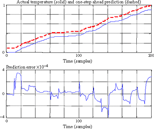
Various architectures, linear and nonlinear, (figure 5) have been tested to estimate an accurate DM model. From these experiments, it has been determined that an OE model having a single linear neuron on the hidden layer is sufficient. To get accurate results (figure 6, the predicted values that are very close to actual values are shifted by 0.1 for clarity), it is necessary to consider the regression vector that consists of n₀ = 7 past estimated temperatures and n₁ = 11 past heat fluxes. The training is based on a unique random sequence that consists of random values of heat fluxes that last 0.1 s. This sequence satisfies the appropriate persistency of excitation conditions for the studied structure. The validation is carried out using 100 random sequences.

Figure 5. Standard architecture for the direct problem.

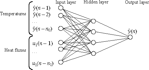
Figure 6. Example of the prediction and prediction error of the model for the direct problem.

The equation of the model can be written as follows (the ‘‘⁁’ indicates an estimated value):

To reverse this equation, it has to be kept in mind that the known values of the inverse model are the temperatures and that the estimated values are the heat fluxes. Knowing that the weights are different from 0, the equation can be reversed as follows:

This is the equation of the first “inverse model”: the MIDM model. It has to be noted that the inversion is possible because the network is composed of linear neurons. It has also to be noted that unlike traditional models, the left-hand side of the representative equation is in advance with respect to the right-hand side of the equation. Hence, to be able to use this equation, it is necessary to know the first ten values of the heat flux. In the following experiments, these values will be set to zero (this corresponds to the example at the beginning of an experiment).

Using the temperatures obtained by the numerical resolution of the direct problem, this model naturally gives quite good results. But using temperatures obtained with a new sequence of heat fluxes can lead to very large errors (figure 7).

Figure 7. Example of results after inversion (for an unknown heat flux sequence).

The simple inversion of the direct model being unsatisfactory, it is necessary to find another way to get an inverse model.

4. The inverse model (DIM model)

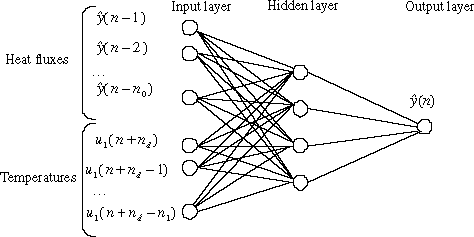
The aim of this part is to find an acceptable representation of the mapping between the temperatures (that are now the inputs) and the heat fluxes (that are now the outputs). As it has been mentioned, it is necessary to take account of a time delay between the temperatures and the heat fluxes. This is done by time-shifting the temperatures. So, the usual architecture of the tested networks is slightly modified (figure 8) by the introduction of the time delay (in terms of samples) n_d.

Figure 8. General architecture of the tested neural networks for the inverse model (DIM model).

A systematic study (similar to the study carried out for the direct model) is carried out considering a large number of values of n₀ and n₁ for the regressors. The couple (temperature response, random sequence) is considered for the learning phase. For the test phase, new random sequences have been used along with two specific sequences: a pulse and a triangle (the latter sequences being often used as tests by many authors, e.g. 8–10,14). For these test sequences, the Euclidean distance between the actual heat flux and the estimated heat flux is computed. The “best” architecture is the architecture that gives the lowest sum of distances. As it is not possible to show here all of the results, only those pertaining to the selected structure are presented (figure 9). This structure has one neuron on the hidden layer; the transfer functions for the hidden neuron and for the output neuron are both linear.

Figure 9. Sum of prediction errors for various time delays.

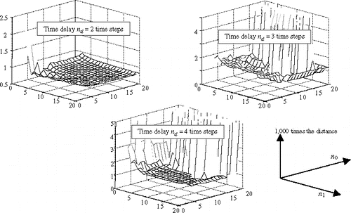
It is clear, from figure 9, that, in the studied case, the best time delay is 2 (0.02 s). Note that a time delay of 1 is impossible to consider; in that case there would be simultaneity of the variations of the input as well as that of the output. The lowest error is obtained using 14 neurons on the input layer (n₁ = 6 for the temperatures, n₀ = 8 for the estimated heat fluxes). The results given hereafter are obtained using this configuration (the predicted values are all shifted by 0.1 for clarity).

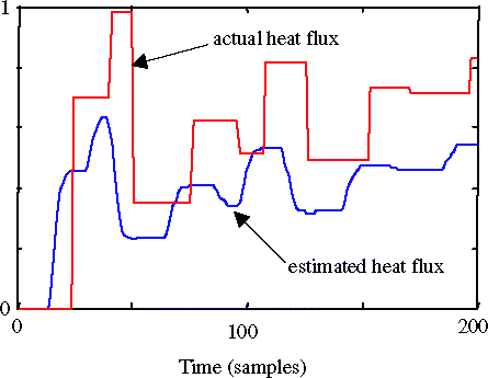
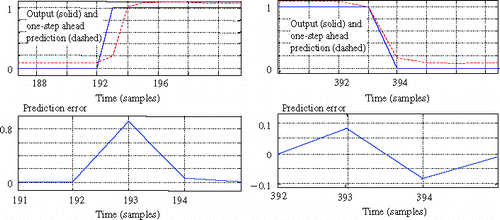
Figure 10 shows that during the test phase the errors are quite small. In the case of the square pulse, this error is located at the fronts. Detailed views (figure 11) show that this error is limited to only three time steps (0.03 s). This is much lower than the time delay that is necessary for the model determined by Kim et al. 9 to get back to a null heat flux (figure 5-b, page 481): about 0.2 s.

Figure 10. Predicted heat flux and prediction errors during the test phase.

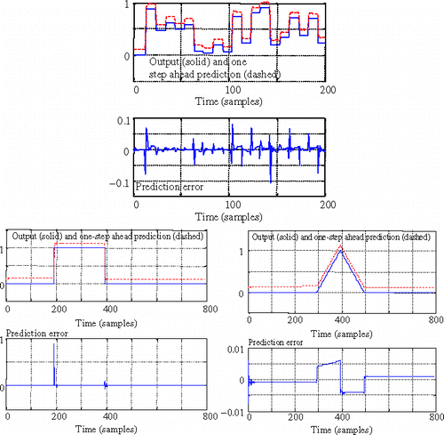
Figure 11. Detailed views of the predicted heat flux and the prediction error for the rectangular pulse.

The learning phase and the test phase have served as a basis for the selection of the suitable architecture. To validate this choice, a first validation is carried out on a new random sequence. Figure 12 shows that good results are obtained (the Root Mean Square Error (RMSE) is about 0.0182).

Figure 12. Prediction error during the validation phase.

Here again it can be seen that the error is limited to very few time steps.

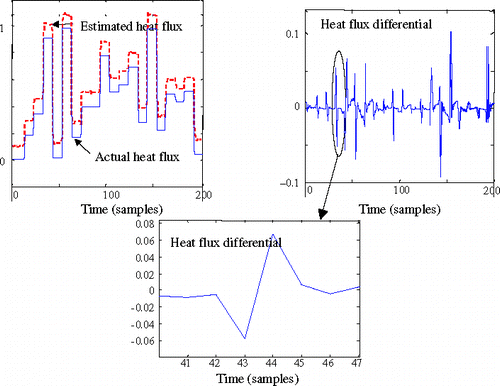
It is well known that inverse problems are generally highly sensitive to noise. It is also well known that neural networks can quite easily handle noisy data. Considering for tests the square pulse, the triangular pulse and a random sequence, a random noise is added to the temperatures (±2%) It is then necessary to train the network using noisy temperatures (noise is also ±2%). Keeping the same architecture, the results are satisfactory. Figure 13 shows the interesting parts of the curves (predicted values are still shifted by 0.1 for clarity). The RMSE is about 0.024 for the random sequence, 0.0179 for the rectangular pulse, and 0.015 for the triangular pulse.

Figure 13. Detailed views of the predicted heat flux and the prediction error when noise is added to the temperatures.

5. Coupling the direct model (DM model) and the inverse model (DIM model)

To show the reliability of the models (direct and inverse), it is possible to couple them. Figure 14 shows a schematic of the configuration.

Figure 14. Coupled neural models for the final validation.

It has been shown that using the mathematical inverse of the direct model (MIDM model) leads to large errors (figure 5). When using the inverse model (DIM model) that has been identified using the temperatures as inputs and the heat fluxes as outputs, the results are much better. Tests have been carried out on 100 random sequences of heat fluxes. An example of the results is given in figure 15.

Figure 15. Comparison of actual and estimated heat fluxes when coupled neural models are used.

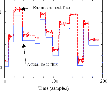
It can be seen that the agreement is satisfactory. To measure the differential, the Root Mean Square Error is calculated (0.0285 for the example shown in figure 15). Figure 16 shows its histogram for the 100 tested cases.

Figure 16. Histogram of the RMSE for the 100 validation cases.

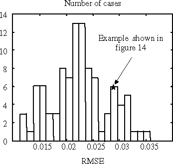
Over the 100 validation cases, the mean RMSE is about 0.0225 (the median being about 0.0223). This shows that the inverse model directly obtained by using a neural network identification process (the DIM model) is accurate and reliable.

6. Conclusions

First, it can be concluded as a general statement and as common sense would advise, that it is preferable to determine the inverse model using the temperature profile (rather than inversing the direct model). It has been shown, on a standard problem, that recurrent neural networks can be used to solve a time-dependent inverse heat conduction problem. It has been shown that for the one-dimensional bar, quite a simple architecture is sufficient (one linear neuron on the hidden layer), but that quite a large number of regressors are necessary, and that the time delay has to be carefully determined. It is foreseen that a much more complicated neural architecture would be necessary for two-dimensional problems.

It can be noted that, once the learning phase is complete (few seconds), the computation time for the estimation of the heat flux is very short (few milliseconds on a 2-GHz personal computer). This confirms the conclusion of Shiguemori et al. 16.

The next steps are as follows:

-	to consider temperature-dependent characteristics of the conducting material,
-	to link the time delay to the size of the studied structure,
-	to address two-dimensional structures.

References

- Shin, M, and Lee, J-W, 2000. Prediction of the inner wall shape of an eroded furnace by the nonlinear inverse heat conduction technique, JSME, Series B 43 (4) (2000), pp. 544–549.
- Reinhardt, H-J, 1993. Analysis of sequential methods of solving the inverse heat conduction problem, Numerical Heat Transfer, Part B 24 (1993), pp. 455–474.
- Yang, CY, 1998. A sequential method to estimate the strength of the heat source based on symbolic computation, Int. J. Heat and Mass Transfer 41 (14) (1998), pp. 2245–2252.
- Lin, S-M, Chen, C-K, and Yang, Y-T, 2004. A modified sequential approach for solving inverse heat conduction problems, Int. J. Heat and Mass Transfer 47 (12–13) (2004), pp. 2669–2680.
- Videcoq, E, and Petit, D, 2001. Model reduction for the resolution of multidimensional inverse heat conduction problems, Int. J. Heat and Mass Transfer 44 (10) (2001), pp. 1899–1911.
- Videcoq, E, Petit, D, and Piteau, A, 2003. Experimental modelling and estimation of time varying thermal sources, Int. Journal Thermal Sciences 42 (3) (2003), pp. 255–265.
- Behbahani-Nia, A, and Kowsary, K, 2004. A dual reciprocity BE-based sequential function specification solution method for inverse heat conduction problems, Int. J. Heat and Mass Transfer 47 (6–7) (2004), pp. 1247–1255.
- Daouas, N, and Radhouani, M-S, 2000. Version étendue du filtre de Kalman discret appliqué à un problème inverse de conduction de chaleur non linéaire, Int. J. Therm. Sci. 39 (2000), pp. 191–212.
- Kim, KY, Kim, BS, Kim, HC, Kim, MC, Lee, KJ, Chung, BJ, and Kim, S, 2003. Inverse estimation of time-dependent boundary heat flux with an adaptive input estimator, Int. Comm. Heat Mass Transfer 30 (4) (2003), pp. 475–484.
- Kim, S, Lee, KJ, Ko, YJ, Chung, BJ, Kim, KY, and Kim, MC, 2004. Direct estimation of time-dependent boundary heat flux, Int. Comm. Heat Mass Transfer 31 (2) (2004), pp. 273–280.
- Chu, SS, and Chang, WJ, 2003. Inverse problems in an axisymmetric multilayer annular cylinder with an interlayer thermal resistance, Int. Comm. Heat Mass Transfer 30 (2003), pp. 379–390.
- Chiwiacowsky, LD, and de Campos Velho, HF, 2003. Different approaches for the solution of a backward heat conduction problem, Inverse Problems in Engineering 11 (6) (2003), pp. 471–494.
- Colaco, MJ, and Orlande, HRB, 2004. Inverse natural convection problem of simultaneous estimation of two boundary heat fluxes in irregular cavities, Int. J. Heat and Mass Transfer 47 (6–7) (2004), pp. 1201–1215.
- Krejsa, J, Woodbury, KA, Ratliff, JD, and Raudensky, M, 1999. Assessment of strategies and potential for neural networks in the inverse heat conduction problem, Inverse Problems in Engineering 7 (1999), pp. 197–213.
- Woodbury, KA, Application of genetic algorithms and neural networks to the solution of inverse heat conduction problems, http://www.me.ua.edu/inverse/NN-GAtutorial/Tutorial-GA-NNrev1.pdf.
- Shiguemori, EH, Harter, FP, Campos Velho, HF, and da Silva, JDS, 2002. Estimation of boundary conditions in conduction heat transfer by neural networks, Tendencias em Matematica Aplicada e Computacional 3 (2) (2002), pp. 189–195.
- Lalot, S, and Lecoeuche, S, 2D localization of a heat source using artificial neural networks. Presented at Proceedings of the HEFAT 2002 Conference. Kruger Park, South Africa, 2002.
- Yilmaz, M, Sengul, M, and Geckinli, M, On the inverse source problem of the Poisson equation. Presented at IJCI Proceedings of International Conference on Signal Processing. September, 2003, (2).
- Haykin, S, 1999. Neural Networks—A Comprehensive Foundation, . Upper Saddle River, New Jersey: Prentice Hall; 1999, Chapters 14 and 15.
- Nørgaard, M, Ravn, O, Poulsen, NK, and Hansen, LK, 2000. Neural Networks for Modelling and Control of Dynamic Systems. London: Springer-Verlag; 2000.
- Lalot, S, and Lecoeuche, S, 2001. Online and offline identification of circulation electrical heaters using neural networks, Transactions of the CSME 25 (3–4) (2001), pp. 277–296.
- Lalot, S, and Lecoeuche, S, 2003. Online fouling detection in circulation electrical heaters using neural networks, Int. J. Heat and Mass Transfer 46 (13) (2003), pp. 2445–2457.
- Pham, DT, and Oh, SJ, 1999. Identification of plant inverse dynamics using neural networks, Artificial Intelligence in Engineering 13 (3) (1999), pp. 309–320.
- Xia, PQ, 2003. An inverse model of MR damper using optimal neural network and system identification, Journal of Sound and Vibration 266 (5) (2003), pp. 1009–1023.
- Ljung, L, 1999. System Identification—Theory for the User, . Upper Saddle River, N.J.: PTR Prentice Hall; 1999.
- Sjoberg, J, 1996. "Non-linear system identification with neural networks". Ph.D. thesis. Sweden: Department of Electrical Engineering, Linköping University; 1996.
- Lalot, S, and Lecoeuche, S, Online identification of circulation electrical heaters as MISO systems using artificial neural networks. Presented at Proceedings of the 35th ASME National Heat Transfer Conference. Anaheim, CA, June 10–12, 2001.
- Nørgaard, M, 2000. "The NNSYSID toolbox for use with Matlab, Version 2". 2000, available on the Internet at: http://www.iau.dtu.dk/research/control/nnsysid.html.