Abstract
Designing the magnetic field distribution and thus the magnetic poles shape and intensity is important in magnetron design and leads to solving the 2D-inverse magnetostatic problem with constraints. This article describes a new regularization approach based on adjusting the size of the Discretization Element in the Source Domain (DESD), a parameter that otherwise is arbitrarily chosen.
A means to relate the size of the DESD to the behavior of the influence matrix is proposed and discussed.
The inverse problem is then reformulated as a three-step algorithm: finding the size of the DESD leading to a well-posed problem; solving the well-posed inverse problem; finding (as a direct problem) the element size that optimizes the approximate solution. Several examples on solving 2D-inverse magnetostatic problems for DESD sizes chosen according to the above analysis are provided.
Results obtained after optimization confirm that the proposed algorithm is efficient, leading to low error levels and providing information on the dimensions of the source domain elements, important for both identification and design problems.
1. Introduction
Solving 2D inverse problems in magnetostatics and electrostatics involves solving systems of linear equations:
(---279--1)
derived from linear Fredholm integral equations of the first kind.
The systems of linear Equationequations (1)(---279--1) are obtained through discretization and co-location of the field generated by the source elements situated in a source domain, onto equally spaced points situated in the area of interest – the mesh area. The influence matrix A obtained for such systems is compact, non-positive-definite, and with a high condition number, making such systems impossible or difficult to solve to an acceptable accuracy level.
Analytic type regularization techniques Citation[1,Citation2] are used to improve the influence matrix coefficients using analytic transformations of the given influence matrix and find a solution within a prescribed error level.
Different types of non-analytical regularization methods have been proposed recently, based on ‘injection of a direct problem’ Citation[3] or on geometry, through a ‘D-optimal design’ Citation[4,Citation5] calculating the source distance to the mesh points that gives the highest determinant value for the matrix A. These types of systems are solved for the suitable distance found, and do not allow for further optimization.
Haueisen et al. Citation[6,Citation7] observed the dependence of the inverse solution accuracy on the size of the triangular boundary-element discretization for applications in electroencephalography, magnetoencephalography, and magnetocardiography.
As the influence matrix coefficients values depend strongly on the size of Discretization Element in the Source Domain (DESD), in this article a new type of regularization is proposed, leading to a reformulation of the problem as a three-step algorithm:
The inverse problem is thus regularized and solved through a three-step algorithm consisting of two optimization problems solved as direct problems and one inverse problem that does not require analytic regularization.
A theoretical proof that an inverse problem can be reformulated as a two-step optimization problem is given by Bruckner et al. Citation[8], their method leading to solving two inverse problems, the first being ill-posed and requiring Tikhonov regularization.
This article proposes a means to estimate the behavior of the influence matrix and the system's convergence as a function of the size of the DESD.
Finding the size of the DESD that leads to a well-posed problem is equivalent to a geometric regularization. Scaling back to find the element size that optimizes the solution gives important information on the actual element size that provides the best resolution in the source domain.
The results obtained for the three-step algorithm are shown for several example cases of magnetostatic inverse problems encountered in planar magnetron design. The numerous numerical experiments we have performed using the three-step algorithm confirm its efficiency. It is not the aim of this article to derive the mathematical proofs for a generalization. We believe that the proposed approach in solving inverse problems by searching for the optimal size of the DESD opens a new direction in the mathematical research for solving inverse problems.
2. The inverse magnetostatic problem
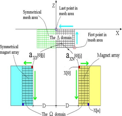
The inverse magnetostatic problem we refer to is encountered in planar magnetrons, where pairs of fixed magnets with opposed polarities are required to generate a constant magnetic field parallel to the OX axis in a certain area (). The shape and intensity of the magnets that generate the above field is to be found (having their direction fixed).
Figure 1. The geometry of a 2D inverse magnetostatic problem for a planar-type magnetron.
The magnets used for this application are made of NdFeB, a material with low demagnetization effect.
The problem can be written as a set of linear Fredholm integral equations:
(---279--2-)
(---279--2-)
with p ∈ Δ, q ∈ Ω, while Br(q) ∈ [ − 1.0, 1.0], where:
| a. | bx (p, q, Br (q)) and bz (p, q, Br (q)) are the magnetic field components on the OX and OZ axes produced by each element (q) of the magnet (source) domain Ω at a point (p) situated in the area Δ; | ||||
| b. | Br (q) is the unknown in the integral equation and it is a characteristic of the magnetic material magnetization (the remanent magnetic flux density) with values in the range of −1.0 T to +1.0 T. | ||||
| c. | Bx (p) and Bz (p) are the required components of the field along the OX and OZ axes at each point p ∈ Δ. | ||||
The field given by each finite size magnet element q can be found from:
(---279--3)
where the magnetic vector potential
(---279----1) can be calculated considering rectangular magnet elements with the magnetic field given by two parallel current sheets of equal current density and opposed direction Citation[9], leading to:
(---279--4)
where
(---279----2) and
(---279----3) are the distances from the point p ∈ Δ to the two current sheets situated at position
(---279----4) and
(---279----5) respectively;
(---279----6) is the width and h is the height of the magnet element cross section.
(---279----7) is the equivalent current sheet density and is related to
(---279----8) for each q ∈ Ω by:
(---279--5)
with
(---279----9) the normal to the current sheet surface.
In the following considerations we take w = h as the size of the DESD.
As the problem is two-dimensional in the plane XOZ, the magnetic vector potential has only the Ay component, and using Equation(4)(---279--4) and Equation(5)
(---279--5) , the magnetic field components become:
(---279--6-)
(---279--6-)
3. Discretization and co-location
Through discretization, the magnet domain Ω is divided into rectangular magnet elements (a magnet array for each magnet pole) indexed by j and the mesh area into equally spaced points indexed by i.
Each pair of symmetrical magnet elements (j) in the arrays will contribute with an influence coefficient aX[i ][ j ] to each mesh point (i); where:
(---279--7)
and the coefficients aXN[i ][ j ] and aXS[i ][ j ] represent the contributions of symmetrical magnet elements from the two magnet arrays with opposed polarities ().
The sum of all magnet element contributions to the magnetic field component on the OX (or respectively on the OZ axis) to a point in the mesh gives the total required field component at that point and forms an equation with X[ j ] – the Br values of magnet elements – as unknowns.
Writing the equations for all the points in the mesh area, the magnetostatic problem Equation(2a(---279--2-) , Equation2b)
(---279--2-) becomes a set of two simultaneous systems of equations with constraints:
(---279--8-)
(---279--8-)
while X(j) ∈ [ − 1.0, 1.0].
The indexes X and Z to the influence coefficients and fields refer to the values on the OX and respectively OZ axis and BX[i ] is the required magnetic field component on the OX axis at the point [i ] of the mesh.
For 2D magnetostatic inverse problems the geometry and in particular the distances between the source elements and the mesh points, as well as the size of the elements in the magnet array (DESD) have an important contribution to the influence matrix coefficients values.
The magnet array and mesh points ordering plays an important role in deciding the properties of the influence matrix and the behavior of the solver. To provide some ordering for the influence matrix we have chosen the geometry shown in .
Considering one of the magnet arrays, the magnet array element closest to the mesh area is the element X[0] and the magnet element that is situated at the largest distance from the mesh area is X[n], where n is the total number of elements in each magnet array. The mesh area elements are ordered in the same manner, their indexing being done as indicated by the arrows in .
The two magnet arrays are symmetrical and with opposed polarities. The symmetry allows solving the problem for only half of each magnet and mesh area thus reducing the number of equations and unknowns.
4. Regularization
Most inverse problems require the use of regularization, as the iterative solvers are not convergent for systems of equations with an influence matrix that has a high condition number, is not positive-definite or has a poor accuracy in the measured or calculated coefficient values.
Through regularization, the influence matrix properties can be improved by:
| a. | –solving the normal system of equations:
where ATA is a symmetrical, positive-definite matrix; or by: | ||||
| b. | applying a regularization technique (Tikhonov) and solving:
where λ is the regularization parameter and IL is an identity operator or a bounded linear operator. | ||||
In the first case most iterative solvers will solve the system, but the solution error for the initial system is higher than the one obtained solving the normal system of equations. The convergence will also be slower, as the new influence matrix ATA has a condition number equal to the square of the condition number of A.
In the second case, finding the optimal value for the regularization parameter is a complicated task, as from the various methods proposed for choosing it, none guarantees an optimal solution and the best method for finding the regularization parameter is still a subject for research in the mathematical field Citation[10–Citation12].
The geometric regularization method proposed in this article is based on finding the size for the DESD that allows stating a well-posed problem (or at least a less ill-posed one) ensuring the convergence of the solver.
By solving the well-posed problem, an approximate solution found will give the ‘pattern’ for the sought magnet array. Then, scanning upon the actual dimensions range, the best error level that can be achieved by that pattern is found.
5. The iterative method
Most used due to their fast convergence, iterative solvers like the Steepest Descent (SD) or Conjugate Gradient (CG) methods need a positive-definite symmetrical matrix in order to be convergent.
In the case of 2D inverse magnetostatic problems most influence matrices are compact, dense, non-symmetrical, and non-positive-definite, so the above solvers cannot be used directly.
As opposed to the SD and CG methods that are considered ‘roughers’ in finding the solution as they approach the solution through large steps (often by getting far from the solution at some stage) elementary iterative solvers like Gauss–Seidel (GS) and its improved versions like Successive Over Relaxation (SOR) or Successive Under Relaxation (SUR) are ‘smoothers’ as they approach the solution through small steps.
The GS and SOR iterative methods are not convergent if the matrix has a spectral radius S(A)>1. As the SUR method with a small relaxation parameter works even when S(A)>1, we have chosen the SUR iterative method to solve these systems.
The advantage in using the SUR solver is that it allows for ‘ups’ and ‘downs’ in the error norm level, being able to avoid being trapped in local minimum.
The SUR iterative method finds at each step:
(---279--11)
and
(---279--12)
where ω is called the relaxation parameter and the SUR method has values for ω<1.
For most of the systems described here, the spectral radius and the optimum relaxation parameter cannot be determined Citation[13]; but its precise value has little influence over the solution as long as it is small enough.
We have chosen ω = 0.001 as a convenient value for this type of iterative systems; ω ≥ 0.01 leads to a loss of accuracy in the solution and ω ≤ 0.0001 leads to a slow convergence.
The SUR method has a fast convergence for systems where an upper and lower limit (constraint) is set for the unknowns. In the following examples, the limits were set for the intensity of the magnet element (Br) between +1.0 T and −1.0 T.
For each unknown, the iteration stops when the value +1.0 or −1.0 is reached – the limit value being assigned to the respective unknown – while the iteration process continues for the rest of the unknowns.
The solution is found when the lowest error norm is reached, or when all unknowns have reached their limit values. The lowest error norm is obtained during the calculation for the solution that has the smallest ‘residual’: r = ∥AX−BX∥.
In general, this is where all iterative solvers choose to stop the calculations, as this is the best solution.
Continuing the calculation until all unknowns have reached either −1 or +1 values, we reach the end of calculation. At the end of calculation the error norm can be higher, but this is not a major problem here, as we rely on the optimization performed at the next step.
6. The DESD size
In most cases, neither the dimensions of the actual source domain or the size of the discretized source domain elements are known, so they are arbitrarily chosen.
The size of the magnet array elements (the size of the DESD) has a strong influence over the convergence of the iterative solver and the solution found.
Even when the solver is convergent, for large size elements the influence of different magnet array elements is overlapping over the mesh points leading to a solution that averages elements’ intensities with high and low values, giving a false solution.
For extremely small size elements, all the elements have the same influence over the points in the mesh as they all have practically the same location (same coordinates), also leading to a false solution.
Considering the above, finding the optimal size of the magnet array elements will make the difference between having to solve a well-posed or an ill-posed problem.
There are no parameters able to provide direct information on the influence matrix behavior from the above point of view and no mathematical theory has yet been developed to relate the convergence behavior of the system to the discretization size in the source domain.
Although it is not the goal of the present article to derive such a theory, we do provide a geometrical interpretation that can give some information on the convergence of the system.
Choosing the geometry presented in the previous chapter we obtain an influence matrix that is ordered such that the coefficients values are decreasing from the first to the last element on columns and also on rows:
(---279--13)
Considering the geometric representation of the solution of a system of n linear equations with n unknowns as the intersection point of the n hyper-planes in the n + 1 dimensional space, the system has a solution only if the hyper-planes are non-parallel.
The coefficients a[i ][0], a[i ][1], … , a[i ][n] on each line in the matrix represent the coordinates of the normal vector to the respective hyper-plane.
The hyper-planes will be non-parallel if the normal vectors are non-parallel: they should not coincide (R1 has to be large and R2 ≈ 1) or if they are close to coinciding (R1 ≈ 1), the slopes should be different or at least calculated with enough precision (R2 has to be large).
We have chosen as global parameters to state the conditions above the norms of the ratios between the most and the least significant coefficient in the matrix on columns R1; and respectively on rows R2.
Therefore, the following norms are considered:
| a. | The norm of the ratio R1 = a[0][ j]/a[n][ j] over the magnet elements (most to least significant element on columns):
| ||||
| b. | The norm of the ratio R2 = a[i][0]/a[i][n] – over the mesh points (most to least significant element on rows):
| ||||
The conditions to be met so that the intersection point exists can be generalized as:
| 1. | The hyper-planes do not coincide (∥R1∥ has a maximum), while the coefficients defining each equation have to be of the same order of magnitude (∥R2∥ has a minimum). | ||||
| 2. | In case the hyper-planes are close to coinciding (∥R1∥ has a minimum) then ∥R2∥ has to have a maximum. | ||||
When ∥R2 = 1∥ the hyper-planes are parallel, so this value is not acceptable.
Too low values for the minimum in each case leads to coincident or parallel hyper-planes and no solution. Too high maxima in each case leads to unstable solutions and lack of convergence for the solver due to divisions by very small or very large numbers.
There is a strong dependence of the ∥R1∥ and ∥R2∥ with magnet array element sizes (the size of DESD) as can be seen from .
Figure 2. The evolution of the ∥R1∥ and ∥R2∥ with the DESD size for the [10 × 20] array situated at 3 distances from the OZ axis: 31 mm, 41 mm, and 51 mm, and a [10 × 30] array (case D) situated at 31 mm from the axis.
![Figure 2. The evolution of the ∥R1∥ and ∥R2∥ with the DESD size for the [10 × 20] array situated at 3 distances from the OZ axis: 31 mm, 41 mm, and 51 mm, and a [10 × 30] array (case D) situated at 31 mm from the axis.](/cms/asset/5c0d14d5-8e62-4b70-8531-79bfd8e4aad6/gipe_a_10051910_f0002.jpg)
According to the conditions stated above the magnet element size h (DESD size) can be chosen as the DESD size where ∥R1∥ has a local maximum and ∥R2∥ has a local minimum; or for a value where ∥R1∥ has a minimum and ∥R2∥ a local maximum, obviously at low element size.
This criterion was used for choosing the size of the magnet array element that would give an influence matrix with a low condition number and then a well-posed problem.
In the following examples the chosen value for the magnet array element size in all situations was h = 1.0 mm.
The influence matrix determined using this magnet element size was used to solve the linear system of equations and find the intermediate solution – the pattern.
7. Results using the three-step algorithm
As the second system Equation(8b)(---279--8-) leads to the trivial solution X[ j ] = 0, we reformulate and solve the problem by splitting it into three steps:
| 1. | choosing the DESD value for the magnet array, as described in the previous chapter; | ||||
| 2. | solving the system of Equationequations (8a) | ||||
| 3. | optimizing the above solution to find the element size that minimizes BZ while it maximizes BX in the same mesh area – looking for a minimum of the ratio BZ/BX (which can be solved as a direct problem). | ||||
The extensive computational experiments we have performed demonstrate that the three-step algorithm leads to an optimal solution of the inverse problem and several examples are presented here.
The problem Equation(8a(---279--8-) ,Equationb)
(---279--8-) was solved for BX = 0.01T in the mesh points for magnet arrays of [10 × 20] elements situated at D = 31 mm, 41 mm, and 51 mm from the OZ axis and 20 mm from the OX axis and an array of [10 × 30] elements at D = 31 mm from the OZ axis and 20 mm from the OX axis.
7.1. Step 1
The choice of the best DESD value is made as explained in the previous chapter and is indicated by arrows in . As can be seen, good choices for the DESD size would be:
| 1. | h = 0.9 mm, (∥R1∥ local minimum and ∥R2∥ local maximum) or h = 1.0 mm (∥R1∥ local maximum and ∥R2∥ local minimum); | ||||
| 2. | h = 1.0 mm (∥R1∥ local minimum and ∥R2∥ local maximum); | ||||
| 3. | h ∈ [1.0, 1.6) mm (∥R1∥ local minimum and ∥R2∥ large); and | ||||
| 4. | h = 1.2 mm (∥R1∥ local maximum and ∥R2∥ local minimum) or h = 0.9 mm (∥R1∥ local minimum and ∥R2∥ local maximum). | ||||
The same initial magnet element size (DESD size): h = 1 mm was chosen for cases (a, b, c) as this value is suitable for these situations. For the situation (d), h = 1.2 mm is the best DESD choice.
The choice of a small value for h leads to a scaling down of the whole magnet array, from the expected size to a smaller one.
7.2. Step 2
The system Equation(8a)(---279--8-) was written for the chosen (DESD) value h and solved for BX field values of 0.01T in the mesh points for the following magnet arrays:
| a. | [10 × 20] elements array at different distances to the OZ axis: (A) 2AX = 0.01 T; D = 31 mm, for h = 1 mm; (B) 2AX = 0.01 T; D = 41 mm, for h = 1 mm; (C) 3AX = 0.01 T; D = 41 mm, for h = 1 mm; (D) 3AX = 0.01 T; D = 51 mm, for h = 1 mm; | ||||
| b. | [10 × 30] elements array at 31 mm to the OZ axis: (E) 3AX = 0.01 T; D = 31 mm, for h = 1.2 mm. | ||||
When writing the scaled down system (for the chosen DESD) the required value for the field in the mesh area has to be scaled down too.
This scaling coefficient appears as a multiplication coefficient at the left-hand side of each system (A, B, C, D, E) and has to have small values, in order to keep the required BX field at high values.
As a solver, it used the SUR iterative method with constraints at +1 and −1 intensity of the magnet elements (maximum Br values) and a relaxation parameter ω = 0.001.
The iteration ends when all the unknowns have reached the constraints (end of calculation).
shows an example on how the error levels at the lowest error norm are affected by a poor choice of DESD dimensions for the system (E).
Figure 3. The relative errors at the lowest norm at mesh points for three values of the chosen DESD size, for the system (E).
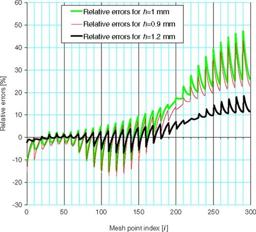
The ∥R1∥ and ∥R2∥ for the system (E) correspond to the situation in .
We notice that for h = 1.0 mm, both ∥R1∥ and ∥R2∥ are large and for h = 0.9 mm ∥R1∥ has a minimum that is high and ∥R2∥ is not on a maximum.
These situations lead to large errors in the final solution and the solution cannot be further optimized.
Choosing h = 1.2 mm, a point where ∥R1∥ has a maximum and ∥R2∥ has a minimum, leads to a solution with a lower error level ().
The level of the solution error found by the SUR solver is not critical, as long as the system is convergent and the absolute relative error level is below 30% – which was the level in the example cases A–E.
This is a major advantage in using the proposed three-step algorithm: the error level required in finding the solution to the inverse problem can be allowed to much higher levels than those required by other regularization methods as the next optimization step will improve it further.
The solution found at step 2 provides the ‘pattern’ for the elements positioning and their intensities, even if it is not the best achievable solution.
Typical solutions at the lowest error norm and at the end of calculation (when all unknowns have reached the constraint values) are presented in .
Figure 4. The solution for the magnet array elements obtained at the lowest error norm (A) and at the end of calculation (B), for a [10 × 20] mesh and a [10 × 20] magnet array situated at 51 mm from the OZ axis. Solutions for the system (D). The +1 and −1 values represent the maximum Br values.
![Figure 4. The solution for the magnet array elements obtained at the lowest error norm (A) and at the end of calculation (B), for a [10 × 20] mesh and a [10 × 20] magnet array situated at 51 mm from the OZ axis. Solutions for the system (D). The +1 and −1 values represent the maximum Br values.](/cms/asset/5b3cbfd0-9787-4440-a19b-54bcd5239331/gipe_a_10051910_f0004.jpg)
We prefer the solution obtained at the end of the calculation (), as it provides a simple geometry and only two values for the intensity of magnet array elements: +1.0 T or −1.0 T (two domains of opposed polarity).
For practical applications, any demagnetization effects that may occur in time will only affect the magnet elements situated at the border of the opposed polarity domains and this can only improve the solution in , as it will tend to get closer to the situation at the lowest norm ().
7.3. Step 3
The objective function in this optimization step is to minimize the ratio BZ/BX over the mesh points for the found solution, thus: minimize ∥BZ/BX∥. The chosen search direction of this minimum is over the DESD size values h.
The BZ[i ]/BX[i ] ratio norm N over the mesh points [i] is:
(---279--16)
Calculating N for the found ‘pattern’ over a range of DESD sizes, a clear minimum can be observed for each magnet pattern obtained by solving the systems A–E ().This minimum represents the size of the DESD where the requested condition ((---279----10) parallel to the OX axis) is best achieved.
Figure 5. The evolution of the BZ/BX ratio norm N with the magnet element size (DESD size) for the solutions found solving the systems A–E.
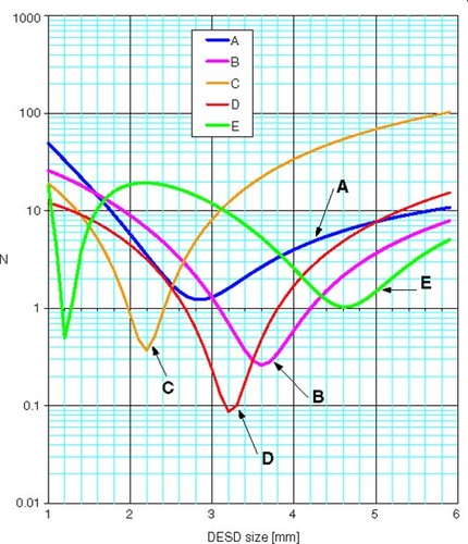
By optimizing the solution looking for a minimum of the BZ/BX ratio, the value for the actual element size (actual DESD size) providing the most accurate solution to both systems Equation(8a(---279--8-) , Equation8b)
(---279--8-) can be found. This optimization improves both BX and BZ values in the required sense.
The search for the DESD size that optimizes the solutions obtained for the systems A–E are presented in . The DESD size corresponding to the minimum of each curve corresponds to the optimized value of the DESD size.
The sharp minima in show how unstable the solution is with the DESD size and how strongly the inverse problem solution depends on the DESD size.
The solution corresponding to (D) is presented in , , , and as linear and 3D graphs of the magnetic field components BX and BZ, the relative errors and the BZ/BX ratio before and after optimization.
Figure 6. Evolution of the BZ/BX ratio in mesh points for the initial and optimized solution, case (D). Optimized DESD size h = 3.2 mm; initial DESD size: h = 1.0 mm.
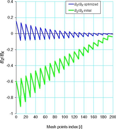
Figure 7. The BX field relative error before and after optimization, at mesh points for case (D). Initial DESD size: h = 1 mm, optimized DESD size: 3.2 mm.
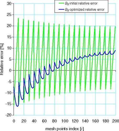
Figure 8. BX field at mesh points after optimization for case (D) at optimized DESD size: 3.2 × 3.2 mm.
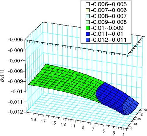
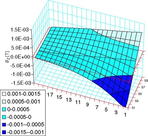
Figure 9. BZ field at mesh points after optimization for case (D) at optimized DESD size: 3.2 × 3.2 mm.
The improvement in the BZ/BX ratio in mesh points after optimization can be observed in ; as well as the improvement in the relative error for the BX field after optimization ().
From relative errors up to 24% for the initial solution – obtained when solving the system for the chosen DESD – the solution reaches relative errors below 10% at most of the points after optimization (for the best DESD size h = 3.2 mm in ).
So, optimization in the sense of minimizing BZ/BX also leads to a decrease of the relative error at mesh points for the BX field.
8. Conclusions
The discussed problem can be stated as a multicriterion synthesis and design optimization problem:
(---279---2)
where AX and AZ are the influence matrices for the fields on X and Z direction. A three-step algorithm is proposed to solve it, together with a new type of regularization.
Defining and discretizing the source domain, together with the way the mesh area is defined through co-location have a tremendous effect on the influence matrix coefficients. Not choosing carefully the size of DESD leads to highly ill-posed problems.
Solving the inverse problem without searching for the optimal DESD size provides a solution that is strictly related to the stated dimensions and cannot be further optimized as it includes the error level imposed by working with an influence matrix whose coefficients are leading to a problem that can be highly ill-posed.
The numerical experiments performed show that it is possible to find a convenient value for the size of the DESD ensuring a less ill-posed problem and the convergence of the solver. The solution found represents a scaling down of the real solution pattern. Scaling up searching for the DESD size that optimizes the solution represents an optimization that leads to a lower error norm.
The search criteria proposed and used to find the best magnet element size – the norms of R1 and R2 over the magnet elements and over the mesh points respectively – provide meaningful and valuable information on the influence matrix behavior and they can be effectively used to analyze and choose the best DESD size.
Depending on the geometry of the system, the requirements for ∥R1∥ and ∥R2∥ can be generalized as: look for a size range where either a large ∥R1∥ or a large ∥R2∥ can be achieved while keeping the other value at low levels.
For source element sizes that do not satisfy the above criteria, the linear system of equations cannot be solved accurately enough or it is not convergent, the problem behaving like an ill-posed problem.
The system cannot be solved or optimized where both ∥R1∥ and ∥R2∥ are high or both low (high condition number), where there is a lack of information (too small size magnet elements, both ∥R1∥ and ∥R2∥ very low) or where the coefficients are not resolved (too large size elements).
The proposed method works best for mesh and magnet arrays with square elements and can be applied for small scaling factors, preferably in the range from 1 to 10.
This geometrical regularization technique is formulated as a three-step algorithm and can be regarded as a reformulation of the inverse problem as a three-step optimization:
The advantage in using this method is that at step 2, the inverse problem is solved as a well-posed (or a less ill-posed) problem and does not require the use of analytical type regularization techniques. Approximate solutions up to 30% relative error level can be used. Moreover, steps 1 and 3 do not necessitate an intense computational effort as they are treated as direct problems.
The proposed algorithm proves to be effective in solving design problems that include a double requirement: the field values are required to have constant values and also to be parallel to one axis in the required region.
This method can also be applied for design problems where only one requirement is imposed, or for field sources identification problems in bio-medical applications. In this case, the condition at the third step can be replaced by: minimize ∥(BX − Breq)/BX∥, where Breq is the required (measured) value of the field; while at the second step, the solution at the lowest error norm should be chosen.
Related Research Data
- Neittaanmäki, P, Rudnicki, M, and Savini, A, 1996. Inverse Problems and Optimal Design in Electricity and Magnetism. Oxford, New York. 1996, New York: Oxford University Press.
- Hanke, M, and Groetsch, CW, 1998. Nonstationary iterated Tikhonov regularization, Journal of Optimization Theory and Applications 98 (1) (1998), pp. 37–53.
- Chadebec, O, Coulomb, J-L, Costa, MC, Bongiraud, J-P, Cauffet, G, and Le Thiec, P, Recent improvements for solving inverse magnetostatic problem applied to thin-shells, IEEE Transactions on Magnetics 38 (2)pp. 1005–1008, March 2002.
- Bégot, S, Hiebel, P, Kauffman, JM, and Artioukhine, EA, D-optimal experimental design applied to a linear magnetostatic inverse problem, IEEE Transactions on Magnetics 38 (2)pp. 1065–1068, March 2002.
- Bégot, S, Hiebel, P, Kauffman, JM, and Artioukhine, EA, 2002. "Computation of Magnetic Field Sources form Measurements Using Iterative Regularization". Rio de Janeiro, Brazil. 2002, Paper presented at the 4th International Conference On Inverse Problems in Engineering.
- Haueisen, J, Bottner, A, Flunke, M, Brauer, H, and Nowak, H, 1997. The influence of boundary element discretization on the forward and inverse problem in electroencephalography and magnetoencephalography, Biomedizinische Technik 42 (1997), pp. 240–248.
- Haueisen, J, Schreiber, J, and Knosche, TR, Dependence of the inverse solution accuracy in magnetocardiography on the boundary–element discretization, IEEE Transactions on Magnetics 38 (2)pp. 1045–1048, March 2002.
- Bruckner, G, and Elschner, J, 2003. A two step algorithm for the reconstruction of perfectly reflecting periodic profiles, Inverse Problems 19 (2003), pp. 315–329.
- Ramo, S, Whinnery, JR, and Van Duzer, T, 1965. Fields and Waves in Communications Electronics. New York, London, Sydney. 1965. p. p. 120.
- Cang, JR, Yeih, W, and Shieh, M-H, 2001. On the modified Tikhonov's regularization method for the Cauchy problem of the Laplace equation, Journal of Marine Science and Technology 9 (2) (2001), pp. 113–121.
- Nair, MT, Hagland, M, and Andersen, R, The trade-off between regularity and stability in Tikhonov regularization, Mathematics of Computation 66 (217)pp. 193–206, January 1997.
- Skipa, O, Nalbach, M, Sachse, FB, and Dössel, O, 2002. Comparison of regularization techniques for the reconstruction of transmembrane potentials in the heart, Biomedical Technology (Berlin) 47 (2002), pp. 246–248, (Suppl. 1).
- Young, DM, 1971. Iterative Solution of Large Linear Systems. New York, San Francisco, London. 1971. p. p. 169.