Constrained optimization of aerodynamic shapes via minimization of total drag

Abstract

In this study, a robust and efficient approach to the multipoint constrained design is developed and applied to the optimization of aerodynamic wings. The objective is to minimize the total drag at fixed lift subject to various geometrical and aerodynamical constraints. The approach employs Genetic Algorithms (GAs) as an optimization tool in combination with a Reduced Order Models (ROM) method based on linked local databases obtained by full Navier–Stokes computations. The work focuses on handling of sensitive nonlinear constraints, such as aerodynamic moments and on the influence of flight conditions on the optimization results. The approach allows us to find optimal points located exactly on the constraints boundary. The results include a variety of optimization cases for two classical wings: a 2D test case of RAE 2822 airfoil and a 3D optimization of ONERA M6 wing. For the considered class of problems, significant aerodynamic gains are obtained.

Keywords:

• Constrained optimization
• Genetic Algorithms
• Aerodynamic shapes
• Reduced-Order Models
• High-performance computing
• Navier–Stokes computations
• 2000 Mathematics Subject Classifications: 76N25
• 76H05
• 76M12
• 80M50

1. Introduction

Robust software for multiobjective aerodynamic optimization through drag minimization is in high demand worldwide. To explain this, consider the task of delivering a payload between distant destinations. Based on the Breguet range equation [1], which applies to long-range missions of jet aircraft, the operator would have to reduce the payload (and thus to reduce the revenue) by 7.6%, to recover the 1.0% increase in drag. Since most airlines operate on small margins, this service most likely will no longer be a profit-generating venture. This illustrates that a 1% delta in total drag is a significant change.

A conventional “trial and error” approach is based on the experience of designers complemented by wind tunnel experiment and Computational Fluid Dynamics (CFD) analysis. The time needed for one optimization loop is measured by months and the whole process may take even years.

That is why, in the last decade, optimal aerodynamic shape design has aroused considerable interest [2–5]. Presently, advanced optimization tools are mostly based on the fully deterministic gradient approach or, alternatively, on the probabilistic evolutionary algorithms. The present state-of-the-art of gradient-based methods can be found in [3], while the overview of nongradient optimization methods is given in [6].

The review of the subject shows that although there has been extensive research on the issue of constrained optimization of aerodynamic shapes, this problem (due to its stiffness) still remains open.

In this context, the main objective of the present research is to create a powerful computational tool for aerodynamic design, which reduces the overall cost of aircraft design and analysis.

The requirements for the computational tool which will be capable of solving the above problem are rather high.

First, the problem of global geometrical representation of aerodynamic shapes still remains open. Second, the construction of a reliable CFD solver suitable for optimization in terms of accuracy and robustness is also not simple. Third, the optimization necessitates high-dimensional search spaces which makes the optimal search highly nontrivial, especially in the presence of nonlinear constraints. Finally, in view of the huge computational volume needed for optimization, stringent requirements should be placed upon the computational efficiency of the whole method.

A CFD solver which drives the optimization process must possess high accuracy of the Navier–Stokes computations on relatively coarse grids, high robustness for a wide range of flows and geometrical configurations, and fast computational feedback.

Note that, for realistic configurations, accurate estimates of sensitive aerodynamic characteristics, such as drag and moments, became available only recently. In particular, this was underlined in the 2nd AIAA Drag Prediction Workshop [7]. The reason is that, for example, drag D is a sensitive functional for the solution of the Navier–Stokes equations, the calculation of which is prone to the loss of significant digits. In order to provide the accuracy of about 1–2 aerodynamic counts needed in engineering context [1], the above solutions must possess very small computational error.

The full Navier–Stokes code NES [8], which employs a high-order low-dissipation scheme within a robust multigrid/defect correction framework, satisfies the requirements of accuracy and robustness. This is indicative of the NES suitability as a CFD driver of optimization process.

In order to satisfy the requirement of fast computational feedback, we propose to scan the optimization search space by using the Reduced Order Models (ROM) approach [9] in the form of Local Approximation Method (LAM) based on local databases obtained by full Navier–Stokes computations (which may dramatically reduce the overall volume of computational work).

Optimization problems in aeronautics necessarily include constraints in their formulation. Unfortunately, the presence of constraints significantly decreases the robustness and the computational efficiency of classical optimization methods. The reason for this is the fact that the calculation of derivatives of the objective function in the vicinity of the constraints boundary is an ill-posed problem which cannot be resolved by the conventional methods.

The situation is especially troublesome in the case of constraints imposed on aerodynamic characteristics (such as aerodynamic moments). The point is that the feasibility of the current geometry (in the context of the above constraints) can be tested only “a posteriori”, that is only through a full CFD run. This means that, in the case of the negative answer (infeasible geometry), the corresponding CFD runs are wasted, and the overall computational efficiency of the optimization algorithm is essentially decreased.

In order to create a robust and computationally efficient optimization tool, Genetic Algorithms (GAs) [11–13] (optimization methods based on coupling deterministic and probabilistic strategies in search of optimum) were employed. A specific feature of the new approach consists of the change in the conventional search strategy. The proposed algorithm employs search paths, which pass via both feasible and infeasible points (contrary to the traditional approach where only feasible points may be included in a path). It is important that the approach allows us to find an optimal point located exactly on the constraints boundary. Contrary to the conventional penalty function method, the proposed approach does not modify the value of the objective function in any feasible point. In a sense, the method is penalty-free and may be labeled as a zero-penalty approach.

The problem of optimization of aerodynamic shapes is very time consuming as it requires a huge amount of computational work. Each optimization step requires a number of heavy CFD runs, and a large number of such steps is needed to reach an optimum. Thus, the construction of a computationally efficient algorithm is vital for the success of the method in engineering environment.

To achieve this goal a multilevel parallelization strategy was used. It includes parallelization of the multiblock full Navier–Stokes solver, parallel evaluation of objective function, and finally, parallelization of the optimization framework.

The method was applied to the problem of multipoint 2D and 3D wing optimization with nonlinear constraints. The results include a variety of optimization cases for two classical wings: a 2D test case of RAE 2822 airfoil and a 3D optimization of ONERA M6 wing. Significant aerodynamic gains were obtained and it was demonstrated that the method retains high robustness of the conventional GAs while keeping CFD computational volume to an acceptable level.

2. Problem formulation

In the case of the single point optimization problem, the objective is to minimize the cost function (total drag coefficient C_D) of a wing subject to the following classes of constraints:

1.	Aerodynamic constraints, such as prescribed constant total lift coefficient (---299----1) and maximum allowed pitching moment (---299----2) : (---299--1)
2.	Geometrical constraints on the shape of the wing surface in terms of properties of sectional airfoils' relative thickness (---299----3) , relative radius of leading edge (---299----4) , trailing edge angle θi: (---299--2)

where i=1,…,N_ws (N_ws – number of sectional airfoils), and values (---299----5) and (---299----6) are prescribed parameters of the problem.

The point design wing must be analyzed over a range of Mach numbers and lift coefficients to ensure the adequacy of the off-design performance. To reach this goal, the multipoint optimization is needed where the objective function is a weighted combination of single point cost functions.

As a gas dynamic model for calculating C_D, C_L and C_M values, the full Navier–Stokes equations are used. Numerical solution of the full Navier–Stokes equations was based on a multiblock code NES [8], which employs structured point-to-point matched grids. The code is based on the Essentially Non-Oscillatory (ENO) concept with a flux interpolation technique [10], which allows accurate estimation of sensitive aerodynamic characteristics, such as lift, pressure drag, friction drag and pitching moment.

The code ensures high accuracy of the Navier–Stokes computations and high robustness for a wide range of flows and geometrical configurations. The high performance of NES was systematically demonstrated by testing it in a wide range of aerodynamic configurations of different complexity: from one-element 2D airfoils (such as NACA0012, RAE2822) through ONERA M6 wing, transport-type supercritical wings and ARA M100 wing-body configuration [8].

The important advantage of the solver NES as a driver of optimization process is its ability to supply reliable and sufficiently accurate results already on relatively coarse meshes and thus to reduce dramatically the volume of CFD computations.

The optimization technique employed GAs in combination with a ROM method based on local databases obtained by full Navier–Stokes computations. The main features of the present multipoint optimization method include a new strategy for efficient handling of nonlinear constraints in the framework of GAs, scanning of the optimization search space by a combination of full Navier–Stokes computations with the ROM method and multilevel parallelization of the whole computational framework, which efficiently makes use of computational power supplied by massively parallel processors (MPP).

3. Constraints handling in genetic algorithms

The GAs are semi-stochastic, semi-deterministic, optimization methods that are conveniently presented using the metaphor of natural evolution: a randomly initialized population of individuals (set of points of the search space at hand) evolves following a crude parody of the Darwinian principle of the survival of the fittest [13].

As a basic algorithm, a variant of the floating-point GA is used. The mating pool is formed through the use of tournament selection. This allows for an essential increase in the diversity of the parents. We employ the arithmetical crossover and the nonuniform real-coded mutation defined by Michalewicz [13]. To avoid a premature convergence of GA, we applied the mutation operator in a distance-dependent form [14]. To improve the convergence of the algorithm we also use the elitism principle.

The optimization method resulted in the following pseudocode:

t = 0

initpopulation P(t)/random/

while not converged do

P* (t): = selectparents P(t)/tournament selection/

recombine P* (t)/arithmetical crossover/

mutate P* (t)/nonuniform + distance-dependent mutation/

evaluate (---299----7) /elitism/

t : = t + 1

enddo

In the considered optimization problem, the presence of constraints has a great impact on the solution. This is because the optimal solution does not represent a local minimum in the conventional sense of the word. Instead, it is located on an intersection of hypersurfaces of different dimensions, generated by linear and nonlinear constraints. Additionally, the problem of finding such an extremum is essentially complicated by the fact that these hypersurfaces, which bound the feasible search space, are not known in advance and may possess irregular topology.

For example, it is quite clear that in the problem defined in Section 2, with no constraints imposed on the airfoil thickness, the optimal profile should be infinitely thin. Thus, it is aerodynamically expected that in the case of the thickness-constrained optimization, the optimal airfoil will possess the minimum allowed thickness. This implies that the optimal point will reside exactly on the corresponding hypersurface.

In the case of constraints, imposed on the aerodynamic characteristics such as pitching moment C_M, the situation is even less controlled. Similar to the previous example, the optimal solution should be located exactly on the constraint boundary. But contrary to the case of geometrical constraints, the determination of the boundary is a much heavier computational problem. For the geometrical constraints, the feasibility test is computationally very cheap while in the case of aerodynamic constraints, the corresponding test requires a full (computationally heavy) CFD run.

Unfortunately, in their basic form, GAs are not capable of handling constraint functions limiting the set of feasible solutions. To resolve this, a new approach is suggested which can be basically outlined as follows (for more details see [15]):

1.

Change of the conventional search strategy by employing search paths, which pass through both feasible and infeasible points (instead of the traditional approach where only feasible points may be included in a path).

2.

To implement the new strategy, it is proposed to extend the search space. This requires the evaluation (in terms of fitness) of the points, which do not satisfy the constraints imposed by the optimization problem. A needed extension of an objective function may be implemented by means of GAs due to their basic property: contrary to classical optimization methods, GAs are not confined to only smooth extensions.

This extension should satisfy only the condition that follows immediately from the main idea to increase the diversity of current population: the objective function in infeasible regions should be defined in such a way that it keeps in the current population a certain number of infeasible individuals, located rather close to the constraints boundary. In such a case we can expect, with rather high probability, that the crossover between feasible and infeasible individuals will produce high-fitness children.

In fact, this allows us to find an optimal point located exactly on the constraints boundary. Contrary to the conventional penalty function method, the proposed approach does not modify the value of the objective function in any feasible point. In this regard, the method implements a zero-penalty approach.

4. Geometrical representation of aerodynamic shapes

An optimization process can be described as a path in the search space, the points of which represent different geometries. Thus, the choice of an appropriate search space is of crucial importance.

In this work it is assumed that:

1.	For the geometry description, the absolute Cartesian coordinate system (x,y,z) is used, where the axes x, y and z are directed along the streamwise, normal to wing surface and span direction, respectively.
2.	Wing planform is fixed.
3.	Wing surface is generated by a linear interpolation (in the span direction) between sectional 2D airfoils.
4.	The number of sectional airfoils Nws is fixed.
5.	Shape of sectional airfoils is determined by Bezier Splines.

The wing planform is defined by the following parameters: the chord length at the root section c₁, span location of the wing sections {z_i} and the corresponding leading and trailing edge sweep angles ((---299----8) and (---299----9) ).

For each wing section, the nondimensional shape of the airfoil (scaled by the corresponding chord) is defined in a local Cartesian coordinate system (---299----10) in the following way. The coordinates of the leading edge and trailing edge of the profile were respectively (0, 0) and (1, 0). For approximation of the upper and lower airfoil surfaces, Bezier Spline representation was used.

Finally, the shape of a sectional profile is completely determined by a total of 2N-5 parameters (---299----11) .

In order to fully specify the wing shape, it is necessary to set locations of the 2D sectional airfoils, in addition to their shapes. Assuming that the chord value and the trailing edge location are defined by the wing planform, sectional locations are specified by means of two additional parameters per section: twist angle (---299----12) and dihedral value (---299----13) . Note that for the root section these values are set to zero.

Thus, the dimension N_D of the search space is equal to: (---299---1) and a search string S contains N_D floating point variables a_j (j=1,…, N_D). The string components are varied within the search domain D. The domain D is determined by Min_j and Max_j values, which are the lower and upper bounds of the variable a_j.

Based on the above approach to the handling of constraints, the modified objective function Q for the solution of drag minimization problem was defined as follows: (---299--3) where each condition is tested independently for all sectional airfoils (i=1,…,N_ws). For 2D optimization, the number of sectional airfoils N_ws=1. In the case of multipoint optimization, the value of C_D represents a weighted combination of total drag values at the flight points participating in optimization.

The choice of constants in equation (3)(---299--3) was based on the principle that their values should be at least several times greater than the upper bound of C_D (about 0.0500 for the considered class of problems). This ensures that, for any feasible point, the value of the objective function will be low in comparison with that of any infeasible point. On the other hand, these constants should not be too high, in order to keep a sufficient number of infeasible points in the population. It appears that the sensitivity of the specific choice is rather low: a change of about 15–20% in the value of the above constants almost has no impact on the final optimal solution.

One of the key difficulties in the implementation of optimization algorithms is due to the fact that, roughly speaking, each CFD run requires a different geometry and, therefore, the construction of a new computational grid. For novel complex geometries, meshes are generally constructed manually, which is very time consuming.

In order to overcome this obstacle and to maintain the continuity of optimization stream, we made use of topological similarity of geometrical configurations (involved in the optimization process), and the grids are constructed by means of a fast automatic transformation of the initial grid, which corresponds to the starting basic geometry.

5. Approximate evaluation of objective function by ROM–LAM method

One of the main weaknesses of GAs lies in their poor computational efficiency. This prevents their practical use in the case where the evaluation of the cost function is computationally expensive as it happens in the framework of the full Navier–Stokes model even in the 2D case.

For example, an algorithm with the population size M  = 100 requires (for the case of 200 generations) at least 20 000 evaluations of the cost function (CFD solutions). A fast full Navier–Stokes evaluation over a 3D wing takes at least 10–15 min of CPU time. That means one step of such an algorithm takes about 3500–4000 h, which is practically unacceptable.

In order to overcome this, we introduce an intermediate “computational agent” – a computational tool which, on the one hand, is based on a very limited number of exact evaluations of objective function and, on the other hand, provides a fast and reasonably accurate computational feedback in the framework of GAs search.

In this study, we use ROM approach in the form of LAM. With the ROM–LAM method, the solution functionals, which determine a cost function and aerodynamic constraints (such as pitching moment, lift and drag coefficients), are approximated by a local database. The database is obtained by solving the full Navier–Stokes equations in a discrete neighbourhood of a basic point positioned in the search space.

In order to ensure the accuracy and robustness of the method, a multidomain prediction–verification principle is employed. That is, on the prediction stage the genetic optimum search is concurrently performed on a number of search domains. As a result, each domain produces an optimal point, and the whole set of these points is verified (through full Navier–Stokes computations) on the verification stage of the method, and thus the final optimal point is determined.

Besides, in order to ensure the global character of the search, it is necessary to overcome the local nature of the above approximation. For this purpose, it is suggested to perform iterations in such a way that in each iteration, the result of optimization serves as the initial point for the next iteration step (further referred to as optimization step).

A brief description of the specific algorithm is given below (for more detail see [15]).

Denote (---299----14) point in the search space, where (---299----15) specify an initial wing shape at nth optimization step, and αⁿ is the angle of attack, corresponding to the prescribed (---299----16) , respectively. Then each wing can be determined by deviations (---299----17) from the coefficients of the initial wing. At fixed values of other flow parameters, the solution functionals depend on the values of (---299----18) and (---299----19) (a deviation from the initial angle of attack). In the optimization process, the following local approximation of a functional Fⁿ is used (subscript n is omitted and F= C_L, C_D, C_M): (---299--4) Here F^o is the functional value at the basic point, and the values Δ F_j (j=1,…N_D) and Δ F_α are determined by means of a mixed linear–quadratic approximation, which employs the local database. One-dimensionally, we use either a one-sided linear approximation (in the case of monotonic behaviour of the solution functionals) or a quadratic approximation (otherwise). (---299---2) (---299---3) Here the following notation is used: (---299---4)

The local database values (---299----20) and F_α are obtained by solving the full Navier–Stokes equations at the corresponding neighbouring points of the basic point in the search space.

6. Computational efficiency of the algorithm

Aerodynamic shape optimization is an example of a highly challenging integral problem. To solve it we need to resolve a number of nontrivial partial problems: (1) to create a robust, accurate and efficient full Navier–Stokes solver, (2) to find an appropriate global geometrical representation of optimized shape and (3) to develop an efficient optimal search able to handle various nonlinear constraints.

Nevertheless, even the successful solution of all three partial problems is not sufficient for the overall success of the optimization algorithm. The point is that the overall computational time needed to obtain the solution is prohibitively high due to significant computational cost of full Navier–Stokes CFD runs and the huge number of the runs.

This means that in order to make the solution practically feasible, it is necessary to significantly improve the computational efficiency of the algorithm. In fact, such an improvement is vital for the success of the method in engineering environment.

This was partially done by decreasing the total number of heavy CFD runs in the framework of the ROM–LAM approach, which allowed us to reduce the computational volume by at least 1 to 2 orders of magnitude. However, the total number of CFD runs still remained very high, which is hardly acceptable even for research purposes.

6.1. Multilevel embedded parallelization

Extensive parallelization is particularly advantageous for achieving a further decrease in the computational volume, since a highly scalable parallel implementation allows the dramatic reduction of the overall computation time.

To reach this goal it was suggested to employ an embedded multilevel parallelization strategy which includes:

1.	Level 1 – Parallelization of the full Navier–Stokes solver
2.	Level 2 – Parallel CFD scanning of the search space
3.	Level 3 – Parallelization of the GAs optimization process
4.	Level 4 – Parallel optimal search on multiple search domains
5.	Level 5 – Parallel grid generation

The first two levels are intended to improve the computational efficiency of the CFD component of the whole algorithm, while the next two levels are needed in order to reach the same goal for the optimization part of the method.

The first level parallelization approach (for a detailed decription see [16]) is based on the geometrical decomposition principle. All processors are divided into two groups: one master processor and N_s slave processors.

The first level of parallelization is embedded with the second level, which performs parallel scanning of the search space and thus provides parallel CFD estimation of fitness function on multiple geometries.

At this level of parallelization (see figure 1), all the processors are divided into three groups: one main processor, N_m master processors and N_m· N_s of slave processors (where N_m is equal to the number of geometries).

Figure 1. Multilevel CFD parallelization. Interconnection of first (main/masters) and second (master/slaves) parallelization levels.

The aim of the main processor is to distribute the set of geometries to be evaluated among master processors, to receive the results of CFD computations from these master processors and, finally, to create local CFD databases. The goal of each master processor is to organize the first level parallelization of the full Navier–Stokes solver corresponding to its own point in the search space (its own geometry).

The third level parallelizes the GAs optimization work unit. At this level of parallelization, all the processors are divided into one master processor with P_s slave processors.

The third level of parallelization is embedded with the fourth level, which performs parallel optimal search on multiple search domains. At this level, all the processors are divided into three groups: one main processor, P_m master processors and P_m·P_s slave processors (where P_m is equal to the number of domains). The interconnection of these parallelization levels is similar to that depicted in figure 1.

The aim of the main processor is to distribute the set of search domains among the master processors, to receive (from these master processors) the results of GA optimization and, finally, to create the set of potential optimal geometries subject to CFD verification. The goal of each master processor is to organize the third parallelization level of GAs search corresponding to its own search domain.

The fifth parallelization level deals with grid generation. At this level, one master-processor and G_s slave processors are employed (G_s is the number of evaluated geometries). The goal of the master processor is to distribute geometries among slave processors, while each slave processor creates a grid, corresponding to its own geometry.

Multilevel parallelization strategy based on the PVM software package was implemented on a cluster of MIMD multiprocessors consisting of 108 (72 HP NetServer LP1000R and 36 IBM Server HS20) nodes. Each node has 2 processors, 2GB RAM memory, 512KB Level 2 Cache memory and full duplex 100Mbps ETHERNET interface. Totally this cluster contained 216 processors with 216GB RAM and 54MB Level 2 Cache memory.

Finally we can conclude that the five-level parallelization approach allowed us to sustain a high level of parallel efficiency on massively parallel machines, and by this way to dramatically improve the computational efficiency of the optimization algorithm.

6.2. Hierarchy principle

An additional source of decreasing the volume of computational work is the use of computational grids coarser than those needed for exact estimations of the objective function. It is feasible if the grid coarsening preserves the hierarchy of fitness function values on the search space (that is, the relation of order is invariant with respect to grid coarsening). This means that the objective function Q_c defined on a coarse grid can be used for solution of the optimization problem, if for every pair of points x₁, x₂ belonging to the search space, the following relation between the values of an objective function Q_c on a coarse grid: (---299--5) implies the same order relation for the objective function Q_f defined on the fine grid: (---299--6)

The applicability of the above principle to the class of optimization problems considered in this article, was validated by comparing the values of lift and drag, computed on grids of different resolutions. It appeared that, for the variety of 2D aerodynamic shapes, the method preserves the hierarchy of drag values for a vast majority of points lying in the parametric space. For each shape, the CFD computations were performed, employing three sequentially refined grids (labeled coarse, medium and fine grids). In the most demanding case, where the coarse grid drag values are compared with those computed on the fine grid, the percentage of the reverse hierarchy is only 3.7% while in the case of the medium/fine comparison, only 5 violations of hierarchy (out of 1225) were found (0.4%). The results reflect the ability of the code to correctly predict the shock position already on the relatively coarse grids. In this context, see also figures 4 and 5, where the comparison between two solutions of the same optimization problem is presented: the first one employed the coarse grid for CFD computations while the second one used the medium grid.

Finally, the cumulative effect of the described techniques allowed to reduce the overall time needed for a one-point 2D wing optimization to 5–6 h on the above described cluster (see Section 6.1). Note that the direct application of the GAs to the solution of the same problem on a single processor from the cluster, requires about 32 years.

7. Analysis of results

The method was applied to the problem of multipoint transonic 2D and 3D wing optimization with nonlinear constraints. The results include a variety of optimization cases for two classical wings: a 2D test case of RAE 2822 airfoil and a 3D optimization of ONERA M6 wing.

7.1. Verification of CFD driver

The CFD solver NES (driver of the optimization process) ensures high accuracy of the Navier–Stokes computations on relatively coarse grids as well as high robustness for a wide range of flows and geometrical configurations. High performance of NES was systematically demonstrated by testing it in a wide range of aerodynamic configurations of different complexities: from one-element 2D airfoils (such as NACA0012, RAE 2822) through ONERA M6 wing, transport-type supercritical wings up to ARA M100 wing-body [8]. This is indicative of the NES suitability as a CFD driver of optimization process.

The results of verification of the NES code for a popular ONERA M6 wing test case are given below. In addition to other reasons, the test case was chosen because the above wing was employed as a starting point in a number of 3D optimizations considered in the present work. The set of computational grids contained three multigrid levels. Each level included 8 blocks. The total number of points in the fine level was close to 200 000.

Figures 2 and 3 present computed surface pressure distribution compared with experiment [17] at a high transonic Mach number M = 0.84, for different span stations. The agreement is reasonably close, which indicates that the computational grid is sufficiently resolved. It is important to emphasize that the NES computation not only favourably compares with experiment but also indicates a good grid convergence.

Figure 2. ONERA M6 wing. Chordwise pressure distribution at wing span station Y = 0.53. α = 3.06^○, M = 0.84, Re=11.72×10⁶. Solid and dashed lines – present computation; crosses – experimental data [17].

Figure 3. ONERA M6 wing. Chordwise pressure distribution at wing span station Y = 0.78. α = 3.06^○, M = 0.84, Re=11.72×10⁶. Solid and dashed lines – present computation; crosses – experimental data [17].

7.2. Optimization of 2D wings

In order to verify the optimization method as a whole, both consistency check as well as comparison with available results of other authors were performed.

The first test case was to find an optimal 12% thickness of 2D airfoil at the design point C_L=0.0, M = 0.6 in the fully turbulent flow regime. Besides the thickness, additional constraints were imposed on the radius of the leading edge and the trailing edge angle.

It is aerodynamically expected that the resulting optimal shape (which corresponds to zero lift) should be symmetric, and the verification of this property is a good test to check the consistency of results. In this connection, in order to make the problem more challenging, a highly asymmetric supercritical RAE 2822 airfoil was chosen as an initial point of the iterative optimization algorithm.

The multigrid set of computational grids contained three levels. The fine, medium and coarse meshes comprised 320×96, 160×48 and 80×24 points in the streamwise and normal to the surface directions, respectively. The optimization problem was solved twice, based on CFD computations employing the coarse and medium grids, respectively. Finally, the aerodynamic characteristics of the optimized airfoils were estimated on the fine grid.

The corresponding results are presented in figures 4 and 5. The optimized aerodynamic shapes vs original RAE 2822 airfoil are shown in figure 4. The resulting optimal profiles are fairly symmetrical in both the cases considered, especially taking into account that the computational meshes originating from the initial asymmetrical airfoil are far from being symmetric. An additional indication to the symmetry of the optimal solution may be found in figure 5, where the surface pressure distribution for the airfoil optimized on the medium mesh is given.

Figure 4. Airfoil shapes optimized on the coarse (1 lev dc) and medium (2 lev dc) grids vs original RAE 2822 profile.

Figure 5. Airfoil optimized on the medium grid at the flight conditions C_L=0.0, M = 0.6. Surface pressure distribution at the design point.

The optimal shapes corresponding to the coarse and medium CFD computations are rather close to one another with values of the total drag coefficient C_D equal to 74.1 and 73.5 drag counts, respectively. Note that even the minimum total drag value of the original RAE 2822 airfoil was about 10 drag counts higher.

To further verify the optimization method, the following multipoint optimization of RAE 2822 airfoil was employed. The main design point was M = 0.734, C_L=0.8, Re=6.5×10⁶ while the secondary design points were: M = 0.754, C_L=0.74, Re=6.2×10⁶ and M = 0.680, C_L=0.56, Re=5.7×10⁶. The target was to minimize a weighted combination of total drag values at these points with the following weight coefficients: w₁=0.5, w₂=0.25, w₃=0.25. The constraints were imposed on airfoil thickness and leading edge radius which cannot decrease. The case served for verification purposes in a number of studies, most recently within the European AEROSHAPE project [19].

The comparison of drag reduction achieved by the current optimization tool OPTIMAS with the corresponding AEROSHAPE results is summarized in table 1.

Table 1. Drag reduction (counts) for multipoint transonic test case. Comparison between current optimization (OPTIMAS) and the results by Quagliarella [19]. 1 aerodynamic count = 0.0001.

Design Point	OPTIMAS	Quagliarella [19]
M = 0.734, CL=0.80	−59.0	−40.0
M = 0.754, CL=0.74	−103.0	−34.0
M = 0.680, CL=0.56	+2.0	+3.0

It can be observed that OPTIMAS achieves an essentially higher drag reduction, especially at the high transonic flight conditions. A detailed analysis shows that this is attributed to a successful shock destruction, which allowed us to eliminate most of the wave drag.

The results presented above indicate an acceptable level of accuracy, robustness and computational efficiency of the proposed optimization method. Essential gains in aerodynamic performance have been achieved in high transonic regime optimizing the RAE 2822 airfoil.

Note that the above airfoil was chosen as the starting point of the optimization, being an established test case, though RAE 2822 is far from being optimal for the considered flight conditions. For this reason, it was interesting to check the performance of the method starting from an airfoil which already possesses a fairly good aerodynamic behaviour at the point of design. We took as the starting point an 18% thickness airfoil which was the result of a multipoint optimization by means of the commercial code MSES [18] at the following two design points: M = 0.6, C_L=0.4 (point A) and M = 0.4, C_L=0.75 (point B). The transition was fixed at 30% of the chord on both upper and lower surfaces.

The current method was applied to the following cases: two single point optimizations (at the above mentioned design points) and a multipoint optimization using a weighted combination of the total drag values at the same points: C_D =  0.6·C_D(A) +  0.4·C_D(B).

The results of the optimization are presented in figures 6–9. In figure 6, the drag polar at M = 0.60 for the original airfoil is compared with those corresponding to the above one- and two-point optimizations, while the aerodynamic shapes at M = 0.40 are presented in figure 7. The surface pressure distributions at point B are shown in figures 8 and 9.

Figure 6. Drag polars at M = 0.60. One-point and two-point optimizations vs original airfoil.

Figure 7. Profile shape. One-point and two-point optimizations vs original airfoil.

Figure 8. Original airfoil of 18% thickness. Surface pressure distribution.

Figure 9. One-point optimization of 18% thickness. Surface pressure distribution.

It may be observed that also in this case, the method (both in one-point and two-point modes) allowed us to obtain a significant improvement of the aerodynamic performance at the design points as well as far beyond them. It is important that the two-point optimization, compared to the one-point optimizations, results in an airfoil shape which possesses an almost identical drag value at point A while the respective value of C_D at point B is only slightly higher.

Note that the analysis of surface pressure distributions shows that the upper surface distribution of the original shape (see figure 8) is not far from a triangular one. In view of aerodynamic common sense, this indicates that the original airfoil is already reasonably good. The optimization at point B leads to a practically triangular distribution (see figure 9).Additionally, it can be observed that the new shape is more rear-loaded than the original one. The two-point optimization retains a triangular form of the upper surface pressure distribution, while the C_p behaviour in the leading and trailing edge areas is closer to the original one.

7.3. Optimization of 3D ONERA M6 wing

Based on the above verification studies (see Section 7.1), it may be concluded that the NES solver supplies accurate asymptotically converged lift and drag coefficients values for transonic 3D wings with grids containing about 193×33 ×33 computational points at the fine level in the streamwise, normal to surface and span directions, respectively. Unfortunately, such computations, though feasible for a single optimization, are too heavy to be used in the industrial framework.

To overcome this limitation, we used the invariance of the hierarchy of objective function values on the medium and fine grids (see Section 6). It appeared that the grids two times coarser in each direction (97 ×17 ×17) satisfy the invariance conditions (5)(---299--5) and (6)(---299--6) . This allowed us to use meshes with such a resolution for optimization purposes.

In the following, we present the results of one- and multi-point drag minimization of ONERA M6 wing at Re=11.72 ·10⁶ and different values of design C_L and Mach numbers representing a wide range of flight conditions. A total of 10 test cases was studied. Design conditions and constraints are summarized in table 2. The corresponding optimal wing shapes are designated by Case_1 to Case_10. In all the optimization cases, the number of wing sections subject to design was equal to N_ws.

Table 2. Optimization conditions and constraints for different test cases.

Case No.	(---299----21)	Design M	Weight	(---299----22)	Nws
1	0.265	0.84	1.0	−∞	2
2	0.500	0.84	1.0	−∞	2
3	0.500	0.86	1.0	−∞	2
4	0.500	0.87	1.0	−∞	2
5	0.500	0.87	1.0	−0.100	2
6	0.500	0.87	1.0	−0.075	2
7	0.500	0.87	0.6	−∞	2
	0.400	0.85	0.4	−∞	2
8	0.500	0.87	1.0	−∞	3
9	0.500	0.87	1.0	−0.100	3
10	0.500	0.87	1.0	−0.100	4

Geometrical constraints on relative thickness, relative leading edge radius and trailing edge angle were kept on a constant level in all the optimization cases: (---299---5)

Note that the value of the relative thickness was not allowed to be lower than that of the original ONERA M6 wing, while the value of the relative leading edge radius was allowed to be lower than the original one.

The design points considered lie in a high transonic Mach range with lift coefficient values varying from moderate to high. At these flight conditions, the flow over the original ONERA M6 wing develops a strong lambda-shock with intensive shock–boundary layer interaction.

The optimization at the design point C_L=0.265, M = 0.84 (Case_1 – moderate target lift coefficient) resulted in the destruction of a strong double-shock, present in the original pressure distribution. This is illustrated by figures 10 and 11, where the pressure distribution on the upper surface of the original wing is compared with that of the optimized one.

Figure 10. Original ONERA M6 wing. Pressure distribution on the upper surface of the wing at M = 0.84, C_L=0.265.

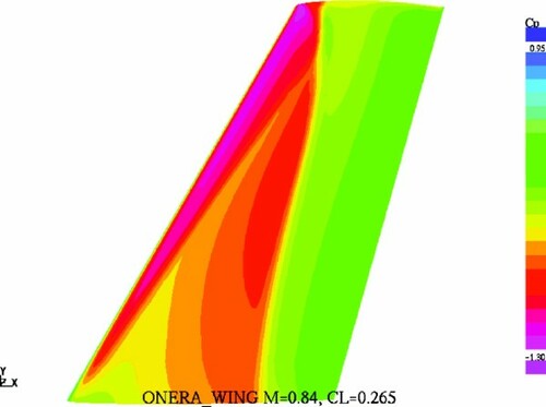
Figure 11. One-point optimization – Case_1. Pressure distribution on the upper surface of the wing at M = 0.84, C_L=0.265.

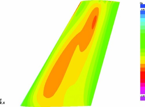
The optimized wing exhibits a shockless behaviour along the whole wing span which led to a significant reduction in the total drag: from 168 to 128 drag counts. Note that the ideal induced drag for the ONERA M6 aspect ratio at C_L=0.265 is equal to 59 counts, and the minimum drag value is equal to about 71 counts for both the wings. Thus it may be concluded that the wave drag contribution to the total drag of the optimized wing is of a minor nature, which is indicative of successful optimization.

At given free-stream Mach and Reynolds numbers, the off-design performance of a wing can be estimated through the lift-drag polar. The corresponding results are presented in figure 12 where the drag polar for the optimized wing (Case_1) is compared with the original one. It is seen that the optimized wing possesses a significantly lower drag not only pointwise but also for all positive lift values. For example, even at the point C_L=0.4, the wave drag rise is estimated by 4 to 5 counts only.

Figure 12. Drag polars at M = 0.84. Original ONERA M6 wing vs. optimized wing (Case_1) at different optimization steps.

Figure 12 also illustrates the convergence of the optimization algorithm (by the example of Case_1). The full convergence was achieved after seven optimization steps, but already after five steps the result was close to the final one. By order of magnitude, such convergence rate is typical of the optimization process for all the test cases considered in this study.

Another important aspect of the off-design performance of wings is their drag rise behaviour at fixed C_L. For Case_1 these data are given in figure 13, where drag polars of the optimized wing for different Mach numbers are shown. It can be assessed that in a wide range of lift values, the drag divergence occurs at least as late as at M = 0.87, which is an essential improvement compared to the original ONERA M6 wing.

Figure 13. Drag polars of the optimized wing (Case_1) at different free-stream Mach numbers.

Now let us analyze the results of optimization at a much more demanding design point characterized by high target lift coefficient at high free-stream Mach number (C_L=0.5, M = 0.87 – Case_4–Case_10).

At these flight conditions, the original ONERA M6 geometry generates a very strong shock which results in a high total drag value (C_D = 544 counts). Similar to the previous case, the optimization allowed us to essentially decrease the total drag down to C_D = 300 counts (Case_4). At this point, the theoretical induced drag for the ONERA M6 at C_L=0.5 is equal to 209 counts, while the minimum drag value is equal to about 87 counts for the original wing. In fact, this is indicative of a very low level of wave drag for the optimized wing.

The corresponding results are presented in figures 14–17, where the pressure distribution on the upper surface of the original wing and chordwise pressure distributions at the midsection of the wing are compared with those of the optimized wing.

Figure 14. Original ONERA M6 wing. Pressure distribution on the upper surface of the wing at M = 0.87, C_L=0.5.

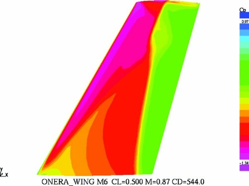
Figure 15. One-point optimization – Case_4. Pressure distribution on the upper surface of the wing at M = 0.87, C_L=0.5.

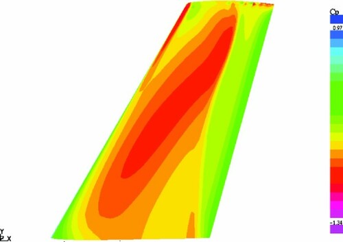
Figure 16. Original ONERA M6 wing. Chordwise pressure distribution at the midsection of the wing at M = 0.87, C_L=0.5.

Figure 17. One-point optimization – Case_4. Chordwise pressure distribution at the midsection of the wing at M = 0.87, C_L=0.5.

The Mach off-design behaviour of the optimized wing (Case_4) is shown in figure 18 where drag polars are computed at different free-stream Mach numbers close to that of the design. The influence of the Mach design value (at the same target C_L) on the off-design performance of optimized wings is illustrated in figures 19 and 20.

Figure 18. Mach off-design behaviour of the optimized wing (Case_4). Drag polars at different Mach numbers.

Figure 19. Mach off-design behaviour of optimized wings. Drag polars at different Mach numbers. Case_3 vs. Case_4.

Figure 20. Mach drag divergence of the optimized wings versus the original ONERA M6 wing. Case_2, Case_3 and Case_4 correspond to design M=0.84, 0.86 and 0.87 respectively.

In figure 19, lift/drag polars for Case_3 (M = 0.86) are compared with the respective curves for Case_4 (M = 0.87) at different Mach numbers: M = 0.84, M = 0.87 and M = 0.90. It is seen that the optimized shapes exhibit a consistent behaviour with the results close to one another in the vicinity of the target C_L at the free-stream Mach numbers lower or equal to 0.87.

Drag rise curves of the wings optimized at C_L=0.5 for different design free-stream Mach numbers are compared to that of the ONERA M6 wing in figure 20. It can be concluded that the optimization allowed us to significantly shift the drag divergence point in the direction of higher Mach numbers and to radically extend the low drag zone. The shift is greater for a greater design Mach number with a small payoff for 0.77 ≤ M ≤ 0.85.

As mentioned above, in the case of 3D optimization there exists an additional class of constraints to be taken into account: the aerodynamic constraints, such as constraint on the pitching moment C_M. This class of constraints is difficult to handle. The point is that the position of test point (trial aerodynamic shape) in the search space with respect to the constraints boundary is not known in advance (contrary to the case of geometrical constraints) which requires a computationally heavy CFD run.

The results of optimization indicate that the present approach is also able to efficiently handle this class of constraints. Several optimization cases, with different values of (---299----23) (maximum allowed value of the pitching moment) were considered. In figure 21 drag polars at M = 0.87 for different (---299----24) are shown.

Figure 21. Lift/drag curves at M = 0.87. ONERA M6 wing vs. one-point optimizations with different values of constraint on the pitching moment. Case_4: no constraint on C_M; Case_5, Case_9 and Case_10: C_M≥ -0.1; Case_6: C_M≥ -0.075.

The unconstrained optimum wing (Case_4) possesses C_M=-0.15 and C_D=300.0 counts at the design point M = 0.87, C_L=0.5. A constrained optimization with (---299----25) (Case_5) achieved a similar drag reduction (C_D=300.5 counts) while for (---299----26) (Case_6) the optimized wing possesses a slightly higher C_D=305.0 counts at the same design point. It is important to underline that up to (---299----27) the total drag of optimized wings is weakly influenced by (---299----28) not only at the design point but also in the off-design zone C_L > 0.3.

Thus the following two conclusions may be drawn. First, the performance of unconstrained pitching moment optimization can be also achieved by a constrained optimization even with a rather significant increase in the maximum allowed value of the pitching moment. Second, the same optimal total drag value C_D may be obtained by markedly different aerodynamic shapes. In other words, the considered optimization problem is ill-posed.

On the whole, it may be also assessed that the incorporation of constraints into the optimization problem is twofold. On the one hand, the presence of constraints (as it was explained above) makes the solution of the optimization problem much more complicated. But at the same time, the constrained problem is more well-posed, which facilitates its solution.

Another important issue is the influence of the parameter N_ws (number of sectional airfoils) on the optimal solution. This is illustrated in figures 22 and 23 where the comparison of the original M6 root and tip shapes with those of wings optimized for different N_ws, is given.

Figure 22. Shape of optimized wings at root section for N_ws=2 (Case_5), N_ws=3 (Case_9) and N_ws=4 (Case_10).

Figure 23. Shape of optimized wings at tip section for N_ws=2 (Case_5), N_ws=3 (Case_9) and N_ws=4 (Case_10).

The analysis shows that, in the middle part of the wing, the optimal shapes tend to possess low curvature immediately outside the leading edge region. For N_ws=2, this leads to a concave form of the above region at the tip section.

In principle, such a shape of the tip airfoil may be infeasible from the design view-point. At the same time, as may be seen from figure 23, the increase in the number of optimized wing sections N_ws leads to a more plausible configuration (especially in the case of N_ws=4).

Airfoil shapes at the midsection of the optimized wings for N_ws=3 and different values of constraint on the wing pitching moment, are shown in figure 24.

Figure 24. Shape of the optimized wings at midsection for different values of constraint on pitching moment. Case_8 – no constraint on C_M; Case_9 – C_M>-0.1. N_ws=3.

Finally, the comparison of lift/drag polars for one-point (Case_4) and two-point (Case_7) optimizations, is presented in figure 25. It is interesting to note that the multipoint optimization allows us to improve the wing performance at low C_L with no penalty at the design C_L values.

Figure 25. Drag polars at M = 0.87. One-point optimization vs. two-point optimization.

8. Conclusions

A robust hybrid GA–ROM approach to the multipoint constrained optimization of aerodynamic configurations is proposed. Main features of the algorithm include an efficient treatment of nonlinear constraints in the framework of GAs and scanning of the optimization search space by a combination of full Navier–Stokes computations with the ROM method, along with an efficient multilevel parallelization strategy, which makes use of computational power supplied by massively parallel processors.

The method was applied to the one-point and multipoint optimization of transonic 2D and 3D wings with a variety of nonlinear constraints. The results demonstrated that the method retains high robustness of conventional GAs while keeping the CFD computational volume to an acceptable level due to a limited use of full Navier–Stokes computations.