Nonlinear inverse unbalance reconstruction in rotor dynamics

Abstract

This article is devoted to the identification and reconstruction of unbalance distributions in an aircraft engine rotor with a nonlinear damping element. We have developed a rotor model that takes into account the nonlinear behavior of a squeeze film damper between the engine's shaft and casing for large oscillation amplitudes. Based on the Tikhonov regularization for nonlinear ill-posed problems, we provided a three-step algorithm that enables us to identify and reconstruct single and distributed unbalances from data measured at the casing of the engine. In view of practical capability, the algorithms were accelerated to meet the requirement of tolerable computation time for larger models, too.

Keywords:

• Rotor unbalance
• Nonlinear damping
• Nonlinear inverse problem
• Tikhonov regularization
• MSC (1991):
• 65R30
• 73D35
• 73D50

1. Introduction

Weight reduction efforts in aeroengine design lead to flexible casing structures, sensitive to vibration excitation from the main rotors. However, the market demands that the smallest possible level of vibrations be transmitted to the aircraft, in order to maximize passenger comfort. This especially holds true for the market segment of long range business aircraft, where engines are generally mounted directly to the fuselage, and low cabin noise and vibration levels are essential in meeting customer expectations. Lowering vibrations caused by unbalances in the rotating parts may also help to increase the safety and lifespan of an aircraft through reducing material fatigue. Since low pressure turbine synchronous vibration levels can be reduced with standard trim balancing methods with relatively little effort and expense, the focus is on reducing vibrations excited by the unbalance distribution on the high pressure (HP) rotor (compressor, turbine and coupling). The HP shaft is not accessible after the engine is assembled, which enforces the principle of ‘right first time’ on balancing and assembly. A direct measurement of HP vibrations in the assembled engine is impossible, due to narrow space, high forces and temperature, therefore we have to rely on indirect measurements and hence have to solve an inverse problem for identifying unbalances in the HP rotor: we are given vibration data, which are measured at a few sensor positions, from which we have to estimate the unbalance distribution.

A good survey of the existing balancing techniques can be found in [1]. The treatment of balancing with inverse problem methods is relatively new. First results on the inverse reconstruction of distributed rotor unbalances from measurements at the casing were achieved in a feasibility study by Rienäcker et al. [2], BMW Rolls–Royce GmbH, and in a cooperation project between Rolls–Royce Deutschland and the AG Technomathematik of the University of Bremen (CERES project, [3]). Both treat the task as a linear problem using a linear whole engine FEM model developed at the BMW Rolls–Royce Group and programmed in NASTRAN for the forward computation. In both cases it was possible to reconstruct continuous unbalance distributions of the same form as bending deformations by linear regularization methods. However, they failed in identifying positions of point unbalances. One possible reason for the failure of this first attempt seemed to be the linearity of the NASTRAN model since it did not take into account nonlinear damping effects arising from squeeze film dampers at the bearing of the rotor (see figure 1). Hence it was our aim to develop a nonlinear model and check if it provides better reconstruction and identification results. As a first step in this direction we did not add non-linear components to the complex NASTRAN model but rather employed a phantom turbine model based on finite element methods for flexible shafts. The parameters of the model were trimmed to meet as characteristic properties of a high pressure rotor of an aircraft engine such as dimensions, eigenforms and resonance frequencies.

Figure 1. Engine interior and mechanical model with squeeze film damper.

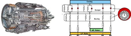
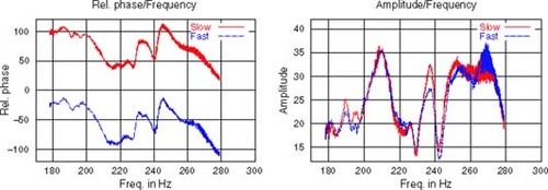
Figure 2. Vibration measurement from a Rolls–Royce turbine.

The solution of the forward problem, i.e., the computation of the vibration of the engine for a given unbalance distribution can be found by solving a nonlinear differential equation. As the forward problem is nonlinear, the inverse problem of identifying unbalances from data measured at certain sensor positions at the housing is nonlinear, too. For its solution, we have used nonlinear Tikhonov regularization. Based on our model for the rotor, we employed a three-step algorithm that enables us to identify and reconstruct continuous as well as discontinuous unbalances (single point unbalances, combinations of point unbalances). All reconstructions were done in the presence of about 15% data error. Our approach has also been adapted to restricted balancing situations, where we are not specifically interested in the unbalance position but rather in a good balancing result with three given positions for balancing masses (as usual in practice). Our approach allows us to compute balancing recommendations (mass and angle) for the admitted balancing positions.

The article is organized as follows: In section 2 we introduce the above-mentioned phantom gas turbine. Details such as the organization of the matrices appearing in the model equation, and physical properties are carefully derived in Appendix A. Section 3 is devoted to the forward problem. Starting from the model equation, we construct a nonlinear operator equation of the form A· f = g describing our problem. Here f denotes the unbalance distribution and g the data measured at the casing of the engine. The solution of the forward problem, i.e., computing g from given f, is contained in this section, too. Section 4 gives a brief introduction to inverse ill-posed problems and their solution. The Tikhonov regularization as one possible solution technique will be introduced. Section 5 is concerned with the inverse problem of determining f from the given (possibly noisy) data g. In particular the derivative of A and its adjoint are computed, which is necessary for applying nonlinear Tikhonov regularization. Moreover, we present a technique for accelerating the minimization of the Tikhonov functional, and derive the reconstruction algorithm in this section. Finally, section 6 contains the results of our test computations and the final three-step algorithm arising from the interpretation of the first reconstruction results. We demonstrate how single and distributed unbalances can be identified and reconstructed, and how the data error influences the reconstructions. We also show how the algorithm works for suggesting balancing corrections if balancing positions are previously fixed.

2. Gas turbine model

In this section we want to establish a gas turbine model based on flexible shafts. Usually such a system is described by an equation of the form (---507--1) where M denotes the mass or inertia matrix, S the stiffness matrix, u the vector of the degrees of freedom of a finite element discretization, p the unbalanced load vector, and Ω the shaft speed. In the presence of damping, and assuming an unbalance f as the causing load, the equation has the form (---507--2) Here D is the sparse damping matrix, f the vector of unbalances and P is a matrix that assigns the forces caused by f to the degrees of freedom in the FEM model.

2.1. Modeling of a flexible shaft using Finite Elements

The usual technique for calculating the dynamic behavior of flexible shafts is the Finite Element Method (FEM). To get an equation of the type (1)(---507--1) , the rotor is divided into separate beam elements (see figure 3).

Figure 3. Flexible shaft, finite beam elements and degrees of freedom.

First of all we will discuss a single beam element. All parameters which refer to a single beam element are marked with a subscript ‘e’. For each node the chosen degrees of freedom have to take into account all geometric boundary and transition conditions. Each finite beam element is treated separately. The motion of the element is described by four shape functions (figure 4). Their scalable amplitudes are the degrees of freedom WL, βL of the left node and WR, βR of the right one. They are ordered by (---507--3) From this ordering results the order of external forces and moments (---507--4) The characteristics of the beam element are given by its stiffness matrix Se, and its inertia or mass matrix Me. The influence of a continuous load is described by the element load vector pe. The element matrices and the element load vector are derived by an energy formulation (see [4]). As mentioned in the introduction, the model parameters are chosen such that the model is very close to the HP rotor of an aircraft engine. With our choice of shape functions, each of the system matrices Se and Me are 4 × 4 real matrices: for a detailed description of these system matrices as well as a derivation of the load vector see Appendix A.

Figure 4. Finite beam elements, loads, shape functions and degrees of freedom.

To build the full system matrices S and M, which combine all beam elements, the element matrices Se [see (A1)], Me [see (A2)-(A4)] resp., are combined by superimposing the elements affecting the right node of the ith element matrix with the ones belonging to the left node of the (i + 1)st element matrix (figure 5). The load vector p is built by superimposing the element load vectors pe [see (A5)] in an analogous manner.

Figure 5. System matrix and superimposed element matrix.

2.2. Gas turbine

The gas turbine shown in figure 6 is modeled as a system of flexible shafts by 44 finite beam elements. Each of the eight disks is modeled by one element; the coupling between the compressor and the turbine consists of two elements. The remaining 34 elements are distributed over the shaft.

Figure 6. Flexible shafts (gas turbine).

Figure 7 shows the first three elastic eigenforms derived from this model. The corresponding eigenfrequencies are 199 Hz (11,940 rpm), 392 Hz (23,520 rpm) and 652 Hz (39,120 rpm). These free–free eigenfrequencies and eigenforms are modified drastically by the turbine's elastic bearings and the housing, which is supported elastically too. To keep the calculation simple, the housing is also modeled as a flexible shaft (figure 8). The bearings are assumed to be isotropic and gyroscopic effects are neglected. Modeling the system this way, the equations of the horizontal plane are decoupled from those of the vertical plane.

Figure 7. Elastic eigenforms and eigenfrequencies (free–free).

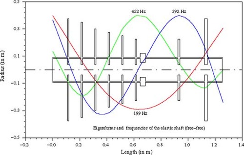
Figure 8. Turbine, housing and elastic bearings.

Since the forces of the elastic turbine bearings are proportional to the relative displacement of the adjacent turbine and housing nodes we have (---507--5) The bearings stiffness s appears at the intersection of the row of the related turbine node with the columns of both involved nodes. Due to Newton's principle of action and reaction, (---507--6) and this has to be inserted in the row related to the degree-of-freedom of the housing. The four coefficients make up a rectangle with positive elements s at the corners on the diagonal, and negative elements −s at the off-diagonal corners. The elastic bearings of the housing are supported by a rigid foundation. So the stiffness appears on the diagonal elements only. The structure of the resulting stiffness matrix S is shown in figure 9.

Figure 9. Block diagonal matrix structure, nonzero off-diagonal elements due to elastic bearings (black squares).

The eigenfrequencies and eigenforms which result from the model in figure 8 are shown in figure 10. Assuming a maximum speed of 17,000 rpm (283 Hz) the turbine crosses two critical speeds at 6060 rpm (101 Hz) and at 8280 rpm (138 Hz). The third critical speed at 17,940 rpm (299 Hz) is not crossed but approached by 95%. The fourth eigenfrequency is found at 22,980 rpm (383 Hz). It is above the range of operating speed. The fifth eigenfrequency at 35,700 rpm (595 Hz) is dominated by movements of the housing.

Figure 10. Eigenforms and eigenfrequencies.

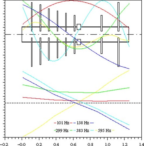
Figure 11. Rotor model with squeeze film damper.

2.3. Model including a nonlinear squeeze film damper

Damping elements are added to the model in the same manner as the elastic bearings. However, the forces of a damper are proportional to the relative velocity of the related turbine and housing nodes. Hence, the related force on the turbine is given by (---507--7) with d being the damping coefficient. The related damping matrix for equation (2)(---507--2) is very sparse. The only nonzero entries make up a rectangle of four entries for each damper as does the elastic bearing for the stiffness matrix.

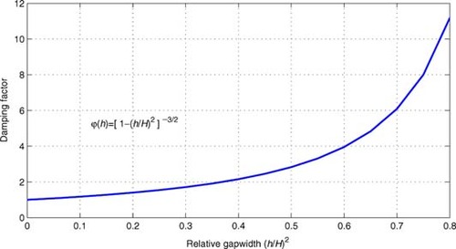
Squeeze film dampers are used to reduce the vibration particularly for nearly undamped aircraft engines. They are best fitted for the reduction of unbalance induced vibrations due to their increasing damping rate at stronger vibrations. Figure 12 taken from [5] shows a schematic of a squeeze film damper. Details shown in figure 13 are taken from [6]. The damping arises from the vibration of the bearing outer ring in a narrow oil-filled gap. The rolling contact bearing is used for separation of the rotating shaft from the nonrotating oil film only. It does not take any static load. The squeeze film damper is a pure damping element. The damping characteristic of a squeeze film damper is nonlinear, when the strength of the damping increases with the level of vibration. A general description of the damping behavior of journal bearings can be found in the related literature. Unfortunately no specific parameters can be given for squeeze film dampers. Only in the special case of circular shaft orbits can the equations of motion be linearized. In the case of infinitesimal vibration, the damping is a function of the oil viscosity and the bearing geometry only. In our calculations, the damping coefficient of the squeeze film damper for higher vibrations was calculated from figure 14 as a multiple of the damping coeffcient related to infinitesimal vibration; see [5].

Figure 12. Schematic of a squeeze film damper.

Figure 13. Details of a squeeze film damper.

Figure 14. Damping characteristic of a squeeze film damper.

3. The forward problem with nonlinear damping

As we consider a model with nonlinear damping provided by a squeeze film damper, equation (2)(---507--2) changes to (---507--8) where D is a function of the solution u. This is due to the fact that the damping of a squeeze film damper depends on the amplitude of the oscillation. The damping is modeled by (see figure 14) (---507--9) with (---507--10) (---507--11) Here H is the maximal gap width in the squeeze film damper, h is the actual gap width, which is the difference between uin, the degree of freedom of the damper position at the shaft, and uout, the degree of freedom of the damper position at the housing. Clearly equation (8)(---507--8) is nonlinear in u, and the solution cannot be computed directly. To simplify the problem, we want to assume that we only have a squeeze film damper at one bearing and constant damping at the other one, hence (---507--12)

3.1. Construction of the forward operator

In this section we model the measurement process. More precisely, we model how an unbalance f in the HP rotor induces vibrations at certain measurement points at the outer surface of the engine. The solution of (8)(---507--8) with (9–12) determines the values for all degrees of freedom at every node of the model. However, measurements can only be taken at certain sensor positions. We want to modify the solution operator of equation (8)(---507--8) in such a way that it maps the causing unbalance vector to the oscillation vector of the nodes at the sensor positions. In the following we assume that we have

1.	s sensors
2.	N sources of unbalance
3.	L degrees of freedom
4.	K frequencies (---507----1) .

3.1.1. The solution operator

As we made an isotropic model, the rotor will move on a circular orbit, and by this we are able to treat the problem in the frequency domain to understand the nonlinear effect of the squeeze film damper instead of performing time-consuming simulations in the time domain. As is normal practice we have defined: (---507--13) For physical reasons we also have (---507----2) , which implies (---507----3) . Inserting (13)(---507--13) in (8)(---507--8) , we get the following equation(s) (---507--14) As (---507----4) we conclude (---507----5) . On the other hand, we have ϕ as a function of u⁺ and u⁻, (---507----6) . Thus (14)(---507--14) is a fixed-point equation for u^±, i.e., (---507----7) .

3.1.2. Real notation

Up to here we have used complex notation in all formulae. Now we want to shift to real notation. The main reason for this change of notation is that convergence results for Tikhonov regularization, which will be used for solving the problem, are only available in the real case. To that end we use the representation (---507---1) This means that we only need u⁺. Denoting (---507--15) (---507--16) (cf (14)(---507--14) ) we get (---507---2) With the additional abbreviation (---507--17) and the notation (---507---3) where the superscript T stands for the transpose, we arrive at the real notation for the solution u of (8)(---507--8) : (---507--18)

3.1.3. The measurement process

We will denote the real formulation of the measured data (---507----8) at frequency Ω and the real formulation of h by (---507--19) (---507--20) Thus we have (---507----9) for the unbalance vector and (---507----10) for the vector of degrees of freedom. Further we assume that

1.	Q1 is the matrix that extracts u at the sensor positions: (---507---4)
2.	Q2 is the matrix that extracts h from ur: (---507---5)

Inserting these definitions in (18)(---507--18) , the forward problem can be written for a fixed frequency Ω as (---507--21) For better readability we will use the abbreviations (---507--22) We remark that for fixed h the above terms are matrices, which have the following sizes: (---507--23) We only have to store the real and imaginary parts of (---507----11) and (---507----12) . An example for those matrices for a specified frequency and h-sample can be found under www.math.uni-bremen.de(---507----13) ramlau\ unbalancematrices.

THEOREM 3.1 Let gr(Ω) be the real data vector containing the degrees of freedom at the sensor positions, h as defined in (11)(---507--11) and (20)(---507--20) , and fr the real notation of the unbalance vector. Then the data vector gr for a given unbalance can be computed by (---507--24) where (---507----14) is defined by (22)(---507--22) .

3.2. Numerical solution of the forward problem

From now on we omit the index r denoting the real notation when no confusion is possible. Solving (---507----15) for given f would be easy if the corresponding h (f) is known. Finding h requires the solution of (---507--25) which again is a fixed-point equation for h. (We refer to (20)(---507--20) for the use of h and h.) Once we have computed h via (25)(---507--25) , the matrix (---507----16) and thus g can be computed immediately. In a first attempt, we have used the classical fixed-point iteration (---507--26) for solving (25)(---507--25) , but found it rather time consuming, since for each hk the matrices (---507----17) have to be computed. Moreover, this process has to be done for each frequency. Even more drastically, the forward problem has to be solved many times when solving the related inverse problem. The present approach is not practicable. Instead, we found the following approach more suitable.

As we have seen above, (---507----18) is a matrix for every given h. Thus, we can precompute for a sample of (---507----19) , (---507----20) , the corresponding matrices (---507---6) and store them in advance. Now for a given unbalance f we only have to pick the matrix which fulfills (at least approximately) (---507--27) A promising fixed-point candidate for (27)(---507--27) is a zero of the real-valued function (---507--28) For finding such a zero hz of p, the function fzero of matlab was employed. It interpolates p and computes an approximative zero of the interpolated function. Thus the algorithm for the forward computation reads as follows:

Table

(---507--29)

(---507--30)

(---507--31)

In all our test computations, the zero of p(hi) was unique, which means that (---507----21) has been correctly identified. In general, the computed value (---507----22) is different from our samples (---507----23) , thus we have used Lagrange interpolation of order two to interpolate the matrices (---507----24) and finally to compute (---507----25) . We have implemented both the classical fixed point method and the above-described method for the solution of the forward problem. Several test computations assured us that they both give the same results, but our approach was much faster.

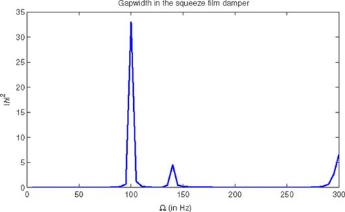
In view of (21)(---507--21) we only have to store the matrix (---507---7) (see (23)(---507--23) ) for each (---507----26) and each (---507----27) . Doing this the entire matrix to be stored is of size (---507----28) . Thus we can handle the forward problem with an acceptable amount of time and storage. Figure 15 shows the movement in the squeeze film damper caused by a real unit unbalance at the third disc.

Figure 15. Forward model: Oscillation in the squeeze film damper. We pass two resonance frequencies at 101 and 138 Hz, and approach a third one at 299 Hz.

4. A short summary on ill-posed inverse problems

In recent years the theory of treating nonlinear ill-posed problems has been well established. For an overview see [7,8]. For the following, let A be a linear or nonlinear operator between real Hilbert spaces. With given data g, we want to find a solution f of the equation (---507--32) The problem is called ill-posed, if the solution f does not depend continuously on the data g. In fact, if we only have noisy data with noise level δ, i.e., (---507----29) , then (provided the inverse A⁻¹ exists) (---507----30) might be an arbitrarily bad approximation to a solution of (32)(---507--32) . To obtain a stable solution, one has to use the so-called regularization methods. The general idea is to approximate the discontinuous inverse operator by a family of continuous operators Tα. The regularization parameter α has to be chosen such that (---507----31) holds. For nonlinear operators, equation (32)(---507--32) might have several solutions. Thus we choose the concept of a (---507----32) -minimum-norm solution, i.e., we are looking for a solution closest to an a priori given function (---507----33) .

A prominent example for a regularization method is Tikhonov regularization. The regularization operator is defined by (---507--33) with the Tikhonov functional given by (---507--34) For the determination of the regularization parameter α, we can use the so-called Morozov's discrepancy principle, where α is chosen s.t. (---507--35) holds [9,10]. In most applications, the exact value of δ is unknown; thus the reconstruction accuracy will depend on a good estimation for δ. In the case of multiple measurements, δ can be estimated by techniques developed in [11]. For linear operators, the minimizer of the Tikhonov functional can be computed by solving a linear system. In the case of a nonlinear operator, optimization methods have to be used additionally to compute a minimizer of (34)(---507--34) . A classical approach to minimize the functional (---507----34) is the use of gradient methods. The gradient of the Tikhonov functional is given by (---507--36) where the linear operator (---507----35) is the adjoint of the derivative of A at the point f [12].

5. The inverse problem for reconstructing unbalances

Knowing the measured data (---507----36) at the sensor positions for each frequency Ω, the inverse problem consists in finding f with (---507--37) and (---507--38) It is well known from the theory of linear damped systems that the reconstruction of the causative unbalance from measured oscillation data is ill-posed. Thus we have to use regularization methods. A widely used algorithm to solve ill-posed inverse problems is Tikhonov regularization, which we have briefly described in section 4. Tikhonov regularization requires the use of an algorithm for the minimization of the Tikhonov functional. For iterative algorithms, the gradient (---507----37) (see (36)(---507--36) ) of the Tikhonov functional with nonlinear operator A plays a central role. For steepest descent methods, (---507----38) is used as a search direction, and for fixed point or Newton's method, a function with (---507---8) is searched for. According to (36)(---507--36) , the computation of (---507----39) requires the knowledge of the Fréchet derivative (---507----40) of A and its adjoint (---507----41) . For our problem we have (---507--39) Here we have shortened the notation of (---507----42) to (---507----43) .

5.1. Derivative of the forward operator and its adjoint

To find a formula for the derivative we have used the Implicit Function Theorem (IFT), which states the following: Provided a function (---507----44) is implicitly defined via (---507----45) , and (---507----46) exists and Fy(x0, y0) is invertible, then y is differentiable in x0 and (---507---9)

THEOREM 5.1 Each component of the Fréchet derivative (---507----47) of A given in (39)(---507--39) is computed by (---507--40) where (---507---10) Thus (---507----48) is a Rank-1 update of (---507----49) .

For a proof of Theorem 2 see Appendix D.

Next we compute the adjoint of the derivative.

LEMMA 1 Each component of the adjoint (---507----50) of (---507----51) given in (39)(---507--39) is computed by (---507--41) For a proof of Lemma 3 see Appendix D.

We remark that in order to compute (---507----52) , we also need to table the matrices (---507---11) with (---507---12) (---507----53) , from which we construct the matrix BΩ, otherwise the computation of (---507----54) would be impossible.

If the derivative is known, gradient-based methods are easily implemented.

5.2. On the minimization of the Tikhonov functional

For the numerical realization of the Tikhonov regularization the minimizer (---507---13) has to be computed. For a linear operator A, this is simply equivalent to solving the linear system (---507---14) For a nonlinear operator A this minimization problem is more demanding. At first, the minimizer of the Tikhonov functional might not be unique anymore, and there might be even only local minimizers. Secondly, the Tikhonov functional is no longer convex. This means in particular that classical algorithms like the steepest descent method can fail to converge to a global minimizer. In [12,13] the so-called TIGRA (TIkhonov–GRAdient)-algorithm was proposed. This method is a combination of Tikhonov regularization and a gradient method for the minimization of the Tikhonov functional. The basic algorithm is as follows:

Table

(---507---15)

Under slight restrictions to the nonlinear operator A it has been shown [13] that this algorithm reconstructs a good approximation to a (---507----55) -minimum-norm-solution (---507----56) of (---507----57) , provided α0 and q are chosen appropriately and a source condition of the form (---507---16) (---507----58) small enough, holds. In this case, an error estimate of the form (---507--42) is obtained. We have used the TIGRA-algorithm for several reconstructions, but found the algorithm rather slow in convergence, which was mainly due to the high number of iterations for the gradient method required for the minimization of the Tikhonov functional for each αk. Thus, our focus was on a replacement of the gradient method by a faster algorithm. First, we want to show that every minimizer of the Tikhonov functional can be characterized as a fixed point of the mapping Φ defined in the following lemma.

LEMMA 2 Every minimizer of the Tikhonov functional fulfills the fixed point equation (---507--43) with (---507--44)

Proof The necessary condition for a minimum of (---507----59) reads (see (36)(---507--36) ) (---507---17) which is equivalent to (---507--45) According to (39)(---507--39) , (---507----60) is a (---507----61) -matrix. By (24)(---507--24) we find that the data g = Af are given by (---507--46) with h = h(f). Looking at (39)(---507--39) , we see that for given (---507----62) , A is a (---507----63) -matrix, and (---507----64) is a (2N × 2N)-matrix.

By the methods presented in section 3.2 we can compute (---507---18) for every given f = f, and thus the matrix (---507--47) is well defined, and equation (45)(---507--45) is equivalent to (---507---19) We remark that the new iteration (---507----65) converged very fast to a minimizer of the Tikhonov functional in all test computations.

5.3. Reconstruction algorithm

Applying Morozov's discrepancy principle, our final algorithm reads as follows:

Table

(---507---20)

A reconstruction of an unbalance distribution from noisy data with the above algorithm needed on average less than 2 min (Matlab implementation, on a PC with 1.33 GHz AMD processor). In comparison, the TIGRA-algorithm needed about an hour for a full reconstruction. As we will see in the following section, the above algorithm did always converge. A convergence analysis of the algorithm is beyond the scope of the present work but is under investigation.

6. Reconstruction results

We have performed a large number of test computations using the following model parameters:

1.	s = 5 sensor positions on the housing [squeeze film damper (1), bearing with constant damping (5), and (2, 3, 4) equidistantly distributed between (1) and (5)]
2.	N = 10 locations of unbalances (compressor: eccentricities at the discs 1 to 6, turbine: eccentricities at the discs 7 and 8, coupling: run out 9, and swash 10)
3.	K = 60 frequencies (---507----66)
4.	a sample of (---507----67) values for (---507----68) : (---507----69)

Given an unbalance or an unbalance distribution, the data g were produced by forward computation. Since it has to be done only once, we have used the (more time consuming) fixed-point iteration (26)(---507--26) . We have disturbed the data with a random additive error of 5% and a random multiplicative error of 15%, and thus obtained (---507----70) . For (---507----71) we have always chosen the zero vector.

6.1. Reconstruction of a single unbalance

First, we have tested our program for several single given unbalances f, namely for an eccentricity at the 2nd disc in the compressor ((---507----72) ), one at the 7th disc in the turbine (f(7) = 0.05 mm), and a run out of the coupling (f (9) = 0.02 mm).

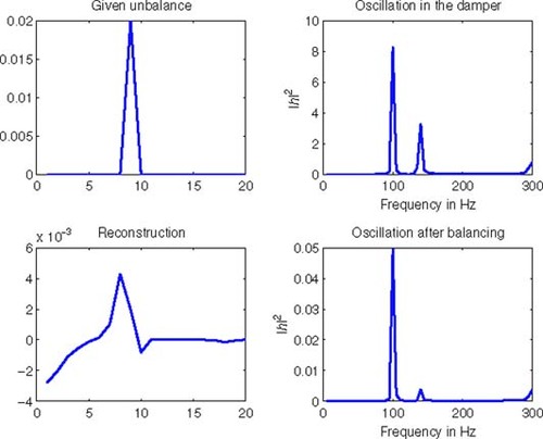
6.1.1. First reconstruction results

We have plotted our reconstruction results in the figures 16 –18. The first picture (top left) always shows the reference unbalance f, the second (top right) its vibration impact at the damper sensor position. In the third picture (lower left) the reconstructed unbalance distribution frec is plotted, and finally picture four (lower right) shows the vibration at the damper sensor position after balancing, i.e., we imagined placing balancing masses according to the reconstructed distribution, meaning we did a forward computation with (---507----73) . Although the results give a hint where the unbalances are situated, the algorithm fails to reconstruct the original unbalance. The reason lies in the following facts. Due to the nature of the measurement process we are working with incomplete data. It is a well known fact from the linear theory of rotor dynamic systems that most information is contained in the resonance frequencies. There are the same number of resonance frequencies as the number of nodes in the model, but usually only the first 10–15 of them are physically reasonable. Using a frequency interval containing all reasonable resonance frequencies, we expect the inverse problem to have a unique solution. However, in practice it is impossible to obtain measurements for all reasonable resonance frequencies and we had to restrict ourselves to an interval that contained two and approaches a third resonance frequency. Different unbalance distributions may produce different vibrations at the sensors within an interval containing all resonance frequencies, but may coincide on the considered subinterval. Thus we have lost the uniqueness of the solution of the inverse problem. Tikhonov regularization with a given (---507----74) reconstructs then a solution closest to (---507----75) . In our case with (---507----76) this means that we end up with a reconstruction for the cause of the unbalance with minimal mass, as can be seen in the figures 16 –18. Although the balancing results are very good, in practice we want to have as few balancing positions as possible due to the costs of the balancing process. Hence the computed reconstructions are not satisfying. To achieve a reconstruction that coincides with the given unbalance we want to locate its position first. To this end we have defined an operator (---507----77) which is a restriction of A to the unbalance positions indicated by (---507----78) , i.e., this operator allows only an unbalance reconstruction at the given positions. These operators can be obtained by extracting the corresponding columns of the matrices A in (39)(---507--39) .

Figure 16. Unbalance at 2nd disc (compressor): reconstruction results.

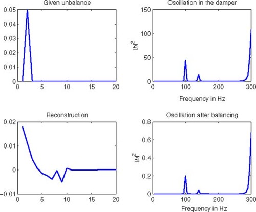
Figure 17. Unbalance at 7th disc (turbine): reconstruction results.

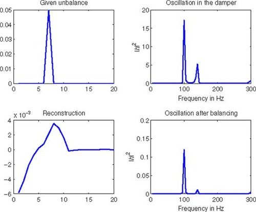
Figure 18. Run out in the coupling: reconstruction results.

6.1.2. Locating of unbalances in compressor, turbine and coupling

As stated above we want to identify the part of the engine (compressor (---507----79) , turbine (---507----80) or coupling = [9, 10]), where the causative unbalance is located. Since we assume that we have single unbalance locations, we can only expect reasonable reconstructions with one of the operators Acomp, Aturb and Acoup. According to the theory of Tikhonov regularization, a necessary condition for a good reconstruction is that the residual (---507----81) is of the same magnitude as the data error δ. As we can see in figure 19, we equal the data error level only with one of the restricted operators while the residua of the others stagnated on a higher level, and conclude that the unbalance can be located only in the part of the engine where the residual with the restricted operator approaches δ.

Figure 19. Residua for compressor, turbine and coupling part, indicating the location of a causing unbalance.

6.1.3. Locating of a single unbalance position

Once the unbalance-causing part of the engine is located, we scan through the possible unbalance positions in order to find the positions where the residuum (---507----83) equals δ. For example, for the 2nd disc unbalance we did reconstructions with (---507----84) . Only by using A[2] does the residuum equal δ, indicating that the unbalance position has been found. With the associated reconstruction (---507----85) , the relative reconstruction error (---507----86) was about 5%. Similar results hold for the other single unbalances; see figure 20.

Figure 20. Identification of unbalance positions in the parts of the engine; residua for the single positions (top), and original and reconstructed unbalance (lower).

6.1.4. General reconstruction approach

The results of the preceding subsections suggest the following general approach to reconstructing a single unbalance:

• Do a minimum-norm reconstruction according to subsection 6.1.1 in order to check the magnitude of the residuum and possible balancing results.

• Identify the part of the rotor where the unbalance is located choosing the part for which the residuum equals δ (cf subsection 6.1.2).

• Scan through the identified part allowing only single unbalance positions for the reconstruction. Again choose the position where the residuum equals δ (cf subsection 6.1.3).

6.2. Reconstruction of an unbalance distribution

To reconstruct an unbalance distribution we have also used the above-suggested approach. In this section we have chosen an eccentricity of 0.05 mm at the 3rd disc in the compressor and a run-out error of 0.02 mm in the coupling. We made a minimum norm reconstruction first in order to get an impression of which reconstruction and balancing accuracy is possible (figure 21). In a second step we compared the residua of the iteration process restricted to the three single parts and combinations of two parts of the engine (figure 22). As a conclusion from figure 22 we presume our unbalances either in the compressor and the turbine or in the compressor and the coupling. It is not very surprising that we cannot identify only a single combination since, for instance, the 7th disc in the turbine is close to the coupling and a balancing weight there will probably have a satisfactory effect in the considered frequency interval.

Figure 21. Reconstruction residuum (lower left) and balancing result (lower right compared to upper right) for an unbalance distribution (upper left).

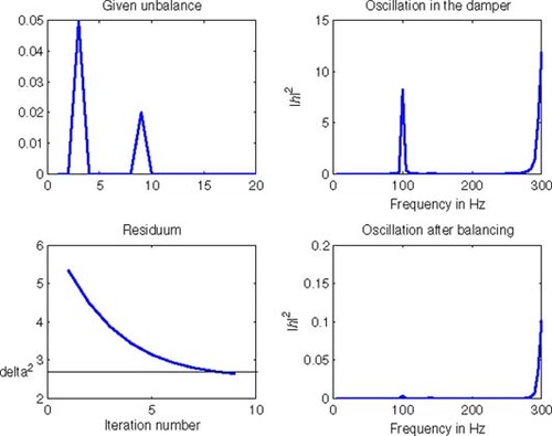
Figure 22. Localization of the parts for an unbalance distribution.

This time the third step is divided. We first allow only single potential unbalance positions and compute the residua (figure 23). We can see that none of the residua approach δ. But when we are looking for a combination of the compressor and one of the other parts, figure 23 recommends trying the positions of disc 1, 2, 3 and 6, since a decreasing of the residuum is visible there. Thus we checked the residua for the restricted operators (---507----87) and plotted the results in figure 24.

Figure 23. Residua squares for the 10 single potential unbalance positions.

Figure 24. Residua squares for combinations of two potential unbalance positions; disc 1, 2, 3 and 6 from the compressor with the remaining positions 7 and 8 from the turbine, and 9 and 10 from the coupling.

Though the residua of some of the combinations came close to δ, only the residuum (---507----88) of the correct combination undercut the δ–level and the iteration stopped. The other residua remained static at a slightly higher level. For the last iterate of the most recommended combinations, we have the following residua (δ² = 2.68): (---507---21) We have to remark that in our case δ is exactly known. For reconstructions with real data, δ has to be estimated. Therefore, it is possible that more than one combination might undercut the estimated δ-level. But due to the regularization theory, the residuum for the right combination tends to zero if α tends to zero. As we can see from figure 24, the wrong combinations remain almost static. The reconstructed unbalance distribution and the balancing result for A[3,9] can be seen in figure 25. The relative reconstruction error (---507----89) is about 7%.

6.3. Balancing at three fixed positions

Due to technical restrictions it is sometimes impossible to place balancing weights according to the reconstructed unbalance distribution. In this case one is only interested in optimal balancing results with respect to given unbalance positions. In practice one often has three fixed positions where balancing weights can be placed. We assumed discs 1, 5 and 8 as such fixed positions and computed the corresponding solution (---507----90) and the balancing result (see figure 26) for the data generated by the above unbalance distribution [3,14]. We can see that the residuum (---507----91) equals δ much faster than the residuum of the A[3,9]-reconstruction (see figure 25). Also the balancing results are much better. For our three-point balancing we got a remaining oscillation in the squeeze film damper of less than 0.3%.

Figure 25. Reconstruction results for A[3,9].

Figure 26. Reconstruction results for A[1,5,8].

6.4. Data error and reconstruction quality

Surely an important item for the unbalance identification accuracy is the quality of the available data. Since we did not have access to real data, we had to revert to simulated data. We have used a reference unbalance at the third disc (f (3) = 0.05), produced the corresponding data by forward computation and disturbed the data with equally distributed random numbers normed to the error level. We varied the error level from 0 to 50%, and applied our three-step algorithm. There was no difficulty in identifying the unbalanced parts of the engine and finally the unbalance position. The reconstructed solution frec was computed using the operator restricted to the 3rd unbalance position A[3]. We defined two measures for the accuracy. The first one is the identification accuracy. (---507---22) Its dependence on the data error level is plotted in the left picture of figure 27. For exact data, the unbalance is exactly reconstructed. The second accuracy measure considers the balancing effect. We compared the oscillation (---507----92) in the squeeze film damper caused by the reference unbalance with the oscillation after balancing with the reconstructed solution (---507----93) (i.e., forward computation with (---507----94) ). The balancing accuracy was defined by (---507---23) The right picture of figure 27 shows the dependence on the data error level. For exact data we have 100% accuracy, i.e., no remaining unbalance after balancing. For 50% data error we have less than 15% remaining unbalance.

Figure 27. Identification and balancing accuracy versus noise level.

7. Summary

In this article, we aim at the development of an algorithm for the reconstruction of unbalances (or its locations) of an aircraft engine from data measured at the engine casing. As we take into account nonlinear damping effects arising from squeeze film dampers at the bearing of the rotor, we have to consider a nonlinear ill-posed problem. The currently used NASTRAN-based models of real engines feature only linear damping effects, and thus we have developed a nonlinear engine model that has the same characteristic parameters as a real engine. Now, the direct problem consists in the computation of the oscillation from given unbalance distributions, while the inverse problem requires the determination of the unbalance distribution from oscillation measurements.

Based on the Tikhonov regularization for nonlinear ill-posed problems, we have introduced a three-step algorithm to reconstruct unbalances in the engine from noisy data. The main idea for a successful identification was the restriction of the reconstruction to parts of the engine or to single unbalance locations and their combinations. The criteria for the correct identification of a position was derived from a discrepancy principle.

The numerical efficiency of our method mainly depends on a fast minimization of the Tikhonov functional. Thus we had developed a fast optimization method for our application, that will guarantee short reconstruction times even for larger models. It turns out that even for noisy data with 15% relative noise our algorithm works successfully. For the first time, point unbalances and discontinuous unbalance distributions could be exactly localized and reconstructed with satisfying accuracy. Additionally, if fixed balancing positions are given, we are able to compute balancing weights for these positions that minimize the remaining oscillations.

The treatment of model errors and a comparison of the linear and the nonlinear model were also under investigation and are topics of a forthcoming paper.

Acknowledgment

The presented work was supported by the BMBF project “Inverse Bestimmung von Unwuchtverteilungen in Flugzeugtriebwerken.”

Appendix

The stiffness matrix was derived as (---507--48) E is Young's modulus, for steel we have E = 208 GPa. For circular section beams, the transverse moment of inertia is given by (---507---24) with dout for the outer diameter and din for the inner diameter of the shaft. The length of the element is represented by L. The shear parameter is given by ([15]) (---507---25) where G is the shear modulus (---507---26) with Poisson's ratio ν. For steel ν equals 0.28. For circular section beams the effective shear area (---507---27) is derived from the area of the cross section (---507---28) and the shear coefficient [16] (---507---29) where (---507---30) The inertia matrix is superimposed of two parts (---507---31) The first part corresponds to the translatorial mass per unit length (---507---32) where ϱ is the density of the material. For steel (---507----95) . We have (see [4]) (---507--49) The second part takes care of the rotational inertia per unit length (---507--50) (---507--51) The element load vector due to continuous load results in (---507--52) where pL denotes the force per unit length at the left node and pR the force per length at the right node.

Suppose we want to determine (---507----96) . We use the Taylor expansion of (---507----97) to determine the derivative from (---507---33) First we have (---507---34) Here (---507----98) is a small term and R(ϵ²) is ‘very small’. We have to determine (---507----99) . This can be done by the following argument where we use the Neumann series (---507----100) . (---507---35) It follows that (---507---36) hence (---507---37)

We want to prove (---507---38) Since (---507----101) and (---507----102) we have (---507---39)

Proof of Theorem 2 We set (---507---40) To extract the derivative of (---507----103) , we consider (---507---41) and conclude from the IFT (---507---42) The partial derivatives were computed as follows (---507---43) and (---507---44) For (---507----104) we have to use Appendix B and the fact that (---507---45) holds. (---507---46) We abbreviate (---507---47) and arrive at (---507---48) As stated in the theorem we have to determine (---507----105) . We use the identity from Appendix C and get (---507---49) So we have (---507---50) and (---507---51)

Proof of Lemma 3 We have (---507---52)