Inverse source identification for Poisson equation

Abstract

A numerical method for identifying the unknown point sources for a two-dimensional Poisson problem from Dirichlet boundary data is proposed. Under an assumption that the total number and estimate positions of the point sources are known, the exact positions and corresponding strengths of the distinct point sources can be identified from scattered (noisy) observed Dirichlet boundary data. Numerical verification indicated that the method is efficient and robust.

Keywords:

• Inverse problem
• Sources identification
• Point mass model
• Poisson equation
• AMS 1991 Subject Classifications:
• Primary 15A29
• Secondary 35J05

1. Introduction

Let Ω be a bounded domain in (---433----1) and Γ:=∂Ω be the boundary of Ω. Consider the following Poisson equation (---433--1) under the Dirichlet boundary condition (---433--2) if f ∈ L²(Ω) and (---433----2) are known, the direct problem specified by (1)(---433--1) –(2)(---433--2) has a unique solution u ∈ H¹(Ω). The aim of this article is to determine the unknown point source function f in (1)(---433--1) from some scattered observed boundary data in (2)(---433--2) : g → f. This is referred as an inverse source identification problem.

Inverse source identification problems are important in many branches of engineering sciences: for examples, crack determination [1,2], heat source determination [3], heat conduction problems [4,5], electromagnetic theory [6], Stefan design problems [7] etc. The investigation of the traditional inverse potential problem can be found in [8,9]. The studies of such problems give a complete analysis of experimental data. In general, a full source f in (1)(---433--1) is not solely attainable from boundary measurements. The inverse source identification problem becomes solvable if some a priori knowledge is assumed. For instance, when one of the products in the separation of variables is known [5,10], or the base area of a cylindrical source is known [10], or a non-separable type is in the form of a moving front [5], the boundary data g can then uniquely determine the unknown sources f. Furthermore, when both u and f are relatively smooth, some standard regularization techniques can be employed (see [11] for a more detailed overview).

It is noted here that for the approximation of a general forcing function, we can use a basis other than the cylindrical function, e.g., the Gaussian function. The cylindrical function to be used in this article, however, is more practical and feasible in view of engineering applications. To simulate the unknown point sources from given Dirac delta functions, we define the following cylindrical functions Φ with base radius ρ > 0 by: (---433--3) Denoting the exact positions of the N distinct point sources by (---433----3) , we now assume that the unknown source function f∈L²(Ω) is a linear combination of Φ in (3)(---433--3) . Furthermore, we prescribe the following conditions on the source function: all point sources are located inside Ω, i.e., (---433--4) Therefore, the source function can be expressed as (---433--5) where |·| denotes the Euclidean distance in (---433----4) . The function f given in (5)(---433--5) can reasonably approximate the weighted sums of the point sources centered at ξ_j with ρ_j ≪ 1, j = 1,…,N.

The approximation (5)(---433--5) is not only appropriate for computation, but also equivalent (up to constant factors) to the logarithmic potential problem with point mass distribution [12,13]. In the logarithmic potential problem, the unknown source function f is determined from observed data in the form of logarithmic potential given by (---433---1) The uniqueness result for the solution had been proven which further justifies our choice of using the cylindrical basis (3)(---433--3) .

In this article, we will establish a numerical scheme for identifying the source strengths and exact positions of the point sources from user-input estimated source locations and scattered boundary data.

2. Methodology for noise-free boundary data

First, we note that the following single source problem (---433--6) has an H¹-solution given by (---433--7) where C(·) is an arbitrary harmonic function in (---433----5) (see [14]).

Following the idea of using fundamental solutions for solving inverse boundary determination problems [15], we express the solution of the multiple point sources model (1)(---433--1) –(2)(---433--2) as a linear combination of the single source solutions with different base radii ρ_j in (7)(---433--7) . The solution to the problem is therefore given by the following superposition (---433--8) where the source strength of the jth point source is defined to be (---433---2) Due to the ill-posed nature of the inverse source identification problem, we assume ρ_j ≪ 1 for all j = 1,…,N so that the cylindrical function Φ in (3)(---433--3) approximates the Dirac delta function. Using the property of (3)(---433--3) , we then have (---433--9) along the boundary Γ where (---433----6) , are arbitrary harmonic functions.

Since the solution on the boundary Γ in (9)(---433--9) depends only on the source strengths and locations, we cannot identify the heights f_j and the radii ρ_j separately. In other words, through observing the boundary data, we cannot recognize the differences between the different shapes of the two cylinders if the volumes of these cylinders are the same.

Note that log |r| completely vanishes when r = 1. We consider this to be a special case when Ω is the unit circle (or a shifted unit circle in general). If the constant term C_j(·) in (8)(---433--8) equals zero, then it is impossible to identify the unknown source if it is located at the center of the circle. In this case, some extra conditions must be imposed: for example, if the overall flux is a constant: (---433--10) then it is sufficient to recover the missing source.

In this article, we will consider the special case of unit circular domain and assume that the overall flux is zero: (---433--11) A constant function (---433----7) for all j = 1,…,N is appended in (9)(---433--9) . If there is a nonzero overall flux, we can set λ = 0 to compute all the source strengths except the one located at the center of the circle. The source strength at the center can be recovered by using the information on the overall flux. This complicated case occurs only when Ω is the unit circle.

Suppose that the set of user-input (estimated) locations of the source points in (5)(---433--5) , (---433--12) is known. Here, ϵ_ξ can be interpreted as the measurement errors of the source positions and treated as an upper bound to all errors in the user-input locations for all j = 1,…,N. It is challenging to identify the unknown source strengths in (8)(---433--8) (i.e., the volume of the cylinder) and their locations (hopefully a better estimation) of the Poisson problem (1)(---433--1) from only scattered Dirichlet boundary data. In the following we first explain the method for the case when noise-free boundary data are available.

Denote Ball(o,r) to be a ball centered at o with radius r and (---433--13) The set (---433----8) must then contain all the exact positions by assumption: (---433---3) Motivated by the method of fundamental solutions [16], we choose a sequence of trial centers, (---433--14) with P ≧ N, and approximate the solution restricted to the boundary (9)(---433--9) by (---433--15) Here, (---433----9) is a constant and σ_k is the (numerical) source strength to (---433----10) .

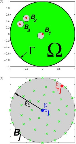
Our goal is to determine the strength sources s_j from the user-input estimated position (---433----11) and the following set of boundary data, (---433--16) where M ≧ P. Refer to figure 1 for the problem setting. As shown in figure 1(a), we consider a case with three source points in Ω and the boundary data are observed at some collocation points in (---433----12) . Figure 1(b) shows the case when the ball (---433----13) defined by (13)(---433--13) contains an exact source position ξ_j. The approximation uses different trial centers (indicated by ×) uniformly distributed in the ball to approximate the Dirac delta source. The union of all these trial centers contained in all balls (---433----14) forms the set (---433----15) in (14)(---433--14) . As shown in figure 1(b), the exact source position ξ_j may not coincide with any of the trial centers.

Figure 1. Graphical display of problem setting. (a) Three exact source positions (•) and their surrounding balls _j centered at some estimated locations. (b) Trial centers (×) in as a circle centered at with radius ϵ_ξ. Here, ξ_j denotes an exact source position and .

We first consider the case when the boundary data in (16)(---433--16) are exact. Collocating (15)(---433--15) at the M distinct collocation points, which are distributed uniformly on Γ or part of Γ, yields (---433--17) where (---433----20) and (---433----21) . The M × P resultant system of (17)(---433--17) has the form (---433--18) where (---433--19) with (---433----22) and (---433----23) denoting the unknown strength sources.

The solution process here is commonly referred as asymmetric radial basis function (RBFs) collocation or simply Kansa's method originated by Kansa [17]. Although the technique introduced by Kansa is very successful in engineering applications, there are no proven results so far for the method. Recently, the asymptotic solvability for a generalized Kansa's method is proven by Ling et al. [18].

Our proposed method does not explicitly require the resultant matrix A to be non-singular. In fact, the resultant A can be extremely ill-conditioned (if not non-singular) due to the ill-posed nature of the problem. In our numerical computations, the resultant system (18)(---433--18) , exactly determined or over-determined, will be solved by using the singular value decomposition (SVD): (---433--20) where U and V are orthogonal matrices and Σ is the diagonal matrix containing the singular values. The stabilized inverse of Σ, denoted by Σ†, is defined to be (---433---4) for i = 1,…,P and some user defined tolerance τ. In other words, any singular value of A with magnitude less than τ will be ignored. The method described above is also commonly referred to as the Truncated singular value decomposition (TSVD) (see [19]).

After computing all the σ_k in (---433----24) by using (17)(---433--17) , we transform the solution in each ball to a single source point. The jth computed source strength associated with each ball (---433----25) _j is then given by (---433--21) which corresponds to the computed location (---433--22) In the computation for each source point, we first obtain the input estimation of location (---433----26) . The proposed method provides an estimate of the source strength by (21)(---433--21) and also gives a new estimation to the source position by (22)(---433--22) . We then regard the output (---433----27) as a new input (---433----28) and continue the computation until a better estimate can be found.

We summarize the methodology for the case of noise-free boundary data g in Algorithm 1 that follows.

3. Methodology for noisy boundary data

For ill-posed problems like the one considered here, computational results are usually very sensitive to errors in the input data. In real-life problems, one can never obtain exact boundary data and hence the investigation for the inverse source identification problem with noisy boundary data is extremely important.

To handle noisy boundary data, we give in the following a mechanism to reject bad trials so that an acceptable approximation to the unknown strengths and source locations can be obtained. As discussed in the last section, the condition (---433----29) indicates a criterion for deciding the computed locations of Algorithm 1.

Table

Algorithm 1 Algorithm for source identification – Noise-free boundary data case.
Ensure: The given N estimated source positions in (12) are distinct in Ω
Ensure: The total number of trial centers in (---433----30) defined by (13) is P
Ensure: A total of M ≧ P boundary data are observed at Γ
for j = 1,…,N do
Place equally distributed trial centers yk in ball (---433----31) j to form the set (---433----32) P as defined in (14)
end for
Compute the resultant matrix by (19)
Compute the unknown source strength associated with (---433----33) by (20)
for j = 1,…,N do
Compute the unknown source strength (---433----34) by (21)
Compute the unknown source position (---433----35) by (22)
end for
RETURN (---433----36) and (---433----37)
Algorithm 2 Algorithm for source identification – Noisy boundary data case.
Given a set of estimate source positions in (12)
Pick a parameter θ such that 1 ≦ θ ≦ 2
while (---433----38) and (---433----39) do not converge do
Observe a new set of noisy boundary data at (---433----40) M
Use Algorithm 1 to obtain the numerical source strength (---433----41) and numerical source position (---433----42)
if (---433----43)
Store (---433----44) and (---433----45)
Compute the mean of the stored (---433----46) and (---433----47)
end if
end while
RETURN (---433----48) and (---433----49)
Algorithm 3 Iterative Algorithm for source identification – Noise-free boundary data case.
While (---433----50) and (---433----51) does not converge do
if First iteration or Strategy 1 then
r:=ϵξ
else if Strategy 2 then
r←r/γ for some constant γ > 0
end if
Use Ball(·,r) to cover the estimated source position
Run Algorithm 1 to obtain numerical source strength (---433----52) and numerical source position (---433----53)
Use current output as new guess: (---433----54) and (---433----55)
end while
RETURN (---433----56) and (---433----57)

On the other hand, it is impossible to further verify the quality of the numerical approximation of Algorithm 1 if only one set of noisy boundary data is available. It is reasonable to assume that the noises contained in (---433----58) _M are white noise and hence the mean of all successive computations are expected to converge to the one found in the noise-free case. This can be achieved by introducing to the procedure in Algorithm 2 with a user-defined parameter 1 ≦ θ ≦ 2 to obtain the following revised algorithm.

The following theorem justifies the convergence of the mean in the revised algorithm.

THEOREM 1 For a fixed set of input locations, if the noise in the boundary data has zero expected value, then the numerical mean computed in Algorithm 2 will converge to the noise-free result.

Proof By assumption, the matrix A in (18)(---433--18) is noise-free. We can write down the resultant system with noise as (---433---5) The mean values (---433----59) implies (---433----60) .▪

In other words, each problem in the noise-free boundary data case will be replaced by a sequence of problems in the noisy boundary data case. Note that the choice of θ has no effect to the proof of Algorithm 2 except the efficiency of the algorithm. The value of θ determines the size of the trust region. If the value of θ is too large, a result of poor estimations in (---433----61) and (---433----62) is expected and hence it affects the convergence of the (---433----63) and (---433----64) . If θ is too small, much more computed results will be classified as poor or unsuccessful and therefore more iterations are needed.

4. Numerical verification

4.1. Noise-free boundary data

In this section, the effectiveness of the proposed computational method will be verified by solving several numerical experiments: In (17)(---433--17) , we take λ = 0.1 in these numerical experiments for simplicity.

Let Ω be the unit disc – the special case. The source function in (5)(---433--5) contains three source points whose exact locations are (---433---6) We demonstrate the performance of Algorithm 1 under two error levels: ϵ_ξ = 0.05 and 0.10. Computation for each test problem was repeated 10 times to avoid the randomness of the input data. The input source locations are randomly chosen such that (---433---7) whose strengths are 3, 4, and −7, respectively.

The computations were performed by using a total of 23 to 346 trial centers in each ball. It was observed that the total number of trial centers plays no role in the convergence of the scheme. This observation agrees with the high convergence rate of RBFs [20] – only a small number of trial centers (or basis) is sufficient to approximate the unknown function. In the following, we only report the numerical result when 102 trial centers were used in each ball.

The boundary data in (16)(---433--16) are exact and the number of boundary data is the same as the number of trial centers, i.e., M = P. In the context of TSVD, one can apply a sophisticated scheme for finding τ. For simplicity, the stabilization parameter for TSVD is chosen to be τ = 10⁻⁴. In general, the approximated source strengths are more sensitive to τ than the source locations. Numerical results are reported graphically in figures 2 and 3.

Figure 2. Numerical results of 10 runs for ϵ_ξ = 0.05 with 10 randomly chosen estimated source positions. (a) Relative error for the computed source strength (ŝ − s)/s. (b) Input position errors and the output position errors .

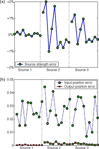
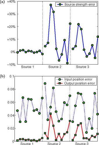
Figure 3. Numerical results of 10 runs for ϵ_ξ = 0.10 with 10 randomly chosen estimated source positions. (a) Relative error for the computed source strength . (b) Input position errors and output position errors .

For ϵ_ξ = 0.05, figure 2(a) indicates that Algorithm 1 is very accurate. The largest relative error over all test runs in the computed source strengths (---433----70) was only (---433----71) . The errors of computed source locations can be found in figure 2(b). Among the 10 test runs, the maximum error in the input positions was 0.0444. It shows that the use of Algorithm 1 reduced the maximum error down to 0.00285. Note that the computational results for Source 1 at [0,0] were more accurate since Source 1 was placed relatively far away from the other two.

For ϵ_ξ = 0.10, however, the computed source strength was not so accurate; see figure 3(a). The relative error in the third run was as large as 37% which, of course, cannot be accepted. However, we observed that Algorithm 1 always improves the estimation of the unknown locations; see figure 3(b).

To improve the accuracy of the result for the case of large location errors ϵ_ξ, we propose an iterative scheme that updates the source positions with the most currently available estimates. Two strategies are imposed to handle the location errors: Strategy 1 uses the initial covering (---433----72) for all iterations without modifications, whereas Strategy 2 reduces the radii of the containing balls in (13)(---433--13) by a factor of γ at every iteration. In comparison to Algorithm 1, the new scheme is less sensitive to the choice of the SVD stabilization parameter τ. The pseudo-code is outlined in Algorithm 3.

For illustration, Algorithm 3 was employed to continue the third run in figure 3. The constant γ in Strategy 2 was chosen to be 2. Results of both strategies are shown in tables 1 and 2. The superscript * in table 2 indicates that a computed source position (---433----73) for this particular iteration was located out of the covering. In this example, this situation occurred at Source 2 where (---433----74) and r = 0.05. The above situation is still acceptable in comparing with figure 1(b).

Table 1. Numerical results of Algorithm 3 – Strategy 1 on noise-free boundary data.

Iteration	Radius of (---433----75)	Max. relative error in (---433----76)	Max. error in (---433----77)
1	0.10	37.1%	0.0424
2	0.10	2.27%	0.00327
3	0.10	−1.62%	0.00275
4	0.10	−2.21%	0.00384
5	0.10	−0.67%	0.00125

Table 2. Numerical results of Algorithm 3 – Strategy 2 on noise-free boundary data.

Iteration	Radius of (---433----78)	Max. relative error in (---433----79)	Max. error in (---433----80)
1	0.10000	37.1%	0.0424
2	0.05000	−11.9%	0.0219*
3	0.02500	−2.64%	0.00432
4	0.01250	−0.0691%	1.05E−4
5	0.00625	−4.62E−3%	1.37E−5

Both Strategy 1 and Strategy 2 showed convergence in this example. Clearly, Strategy 2 showed faster convergence than Strategy 1. On the other hand, we do not have a robust strategy or any theoretical justification for picking the value γ. In fact, there will be a problem in using Strategy 2 when the value of γ is too small such that some exact source positions no longer lie in the balls. A hybrid of these strategies should be considered: reduce r (as in Strategy 2) only if convergence in Strategy 1 is detected.

4.2. Noisy boundary data

Although the study of exhaustive numerical examples is not within the scope of this article, our intention here is to provide some insights about the performance and behavior of Algorithm 2.

Consider the same problem given in section 4.1 but now with position error ϵ_ξ = 0.05. The total number of collocation points was taken to be twice as much as the number of trial centers, i.e., M = 2P. The input locations were (---433---8) with maximum location error 0.0434. The parameter θ in Algorithm 2 was chosen to be 2. Random errors with different noise levels were added to the boundary data for each iteration. Again, Algorithm 2 was repeated for 10 successful runs. The numerical results are listed in table 3 where the total runs indicates the number of test runs in order to have 10 successful runs. As the error level increased, more runs were required as expected. The maximum (relative) error in the (---433----81) increased rapidly with the increase in noise level. In conclusion, improvement in location estimation for all tested noise level had been observed. Note that one can improve the performance of Algorithm 2 by introducing the iterative strategy as given in Algorithm 3 and an adaptive strategy in choosing θ.

Table 3. Numerical results for Algorithm 2 on noisy boundary data.

Noise level	Total runs	Max. error in mean((---433----82) )	Max. error in mean((---433----83) )
0.01	10	−3.25%	0.0101
0.03	14	14.6%	0.0159
0.05	16	29.1%	0.0340

Let us consider the worst case in table 3 when the noise level in boundary data was 0.05. Suppose that (for some reason) we believe the result based on ten successful runs was trustworthy. Motivated by Algorithm 3, we can take the output (---433----84) as a new guess position and reduce the radius of each ball (---433----85) _j to ϵ_ξ/2 = 0.025. It was observed that (---433----86) for some j as the maximum error in position was 0.0340 according to table 3. Without any a priori knowledge, a similar situation will very likely happen in practice. The results after running Algorithm 2 for another 10 successful runs are: (1)(---433--1) the maximum error in the source strength (---433----87) was 3.02%, which was comparable to the best case in table 3; and (2)(---433--2) the maximum error in the position (---433----88) was 5.10E−3, which was the best result among all estimations found in table 3. Due to the poor placement of some (---433----89) _j, several good runs were rejected. A total of 26 total runs were taken before having the required successful runs.

From the numerical experiments, we found that even with the presence of noise in the boundary data, the proposed method can actually capture both the source strengths and their exact locations.

4.3. Example with 6 source points

Finally, we gave the results of Algorithm 3 with 6 source points: (---433---9) where the source strengths equal (---433---10) All parameters remained the same as in the previous example, except that the coefficient λ in (17)(---433--17) was set to 0 to reflect the fact that the sum of source strengths is not equal to zero. The computation by Algorithm 3 was repeated for 5 iterations and the results for noise levels ϵ_ξ = 0.05 and ϵ_ξ = 0.10 are displayed in tables 4 and 5, respectively. The results are all comparable with table 1 (the case of 3 source points).

Table 4. Numerical results for problem with 6 source points and ϵ_ξ = 0.05.

Iteration	Radius of (---433----90)	Max. relative error in (---433----91)	Max. error in (---433----92)
1	0.05	−3.38%	0.0114
2	0.05	−0.213%	0.00131
3	0.05	0.035%	2.04E−4
4	0.05	0.030%	1.41E−4
5	0.05	0.029%	1.37E−4

Table 5. Numerical results for problem with 6 source points and ϵ_ξ=0.10.

Iteration	Radius of (---433----93)	Max. relative error in (---433----94)	Max. error in (---433----95)
1	0.10	−8.45%	0.0244
2	0.10	−0.667%	0.00545
3	0.10	0.263%	8.57E−4
4	0.10	0.191%	4.76E−4
5	0.10	0.177%	5.43E−4

5. Conclusion

We proposed a numerical method for inverse source identification problem for Poisson equation. The method only requires estimated locations of source points and scattered Dirichlet boundary data (with noise) to compute both the unknown source strengths and locations.

Numerical experiments indicated that the proposed algorithms are robust and accurate. In fact, if the algorithms converge, the results are very accurate. Most importantly, the algorithms allow high tolerance to wrong algorithmic decisions which makes the method practical to handle real-life problems.

Acknowledgments

The first author was supported partially by a Postdoctoral Fellowship from the Japan Society for the Promotion of Science. The work of the second author mentioned in this article was fully supported by a grant from the Research Grants Council of the Hong Kong Special Administrative Region, China (Project No. CityU 1185/03E). The third author was supported partially by Grant 15340027 from the Japan Society for the Promotion of Science and Grant 15340015 from the Ministry of Education, Cultures, Sports and Technology.