FIR-type and IIR-type neural networks, and their application to shape optimization of a magnetic pole

Abstract

This article presents two types of neural network (NNs), Finite Impulse Response (FIR) and Infinite Impulse Response (IIR) and their application to a magnetic pole shape optimization problem. To begin with, the architecture and the learning algorithm of the two types of the NN are provided, and then their application to the magnetic pole shape optimization problem is presented. The feature of the two networks is that they have delay elements within the network, which act as a memory function that stabilizes the back propagation learning process calculation. The conclusions obtained showed that these NNs could reduce the iteration process when compared to the conventional feed forward type NN, and the learning iteration for the convergence of the IIR network is less than that of the FIR network.

Keywords:

• Neural network
• Shape optimization
• Digital signal processing
• Magnetic field analysis

1. Introduction

Neural networks (NNs) have a wide range of applications, such as signal processing, image processing and control system design because of their flexible computing ability. Besides these applications, the NN is useful for the optimization problem. Particularly, the shape optimization problem of magnetic pole using NN has been taken up from the viewpoint of the flexible pattern recognition function of the NN [1–3]. However, one of the drawbacks of the NN is the long period of time required for training in the back propagation (BP). In order to reduce the training time, the momentum method and the combined Kalman filter are reported to be useful for the learning of the NN [4–6]. Furthermore, FIR-type and IIR-type NNs are presented as techniques for further improvement of the BP learning process of the NN [7,8].

First, this article provides the architectures of the FIR-type and the IIR-type NNs, and then the formulation of algorithm based on the BP learning process of the networks. The common feature of both NN is that they have memory elements. In other words, the FIR-type network has the delay elements for the input side, and the IIR-type NN has the delay elements for the input and output side. The delay elements act as memory functions, which have an influence on the learning process.

Second, this article presents the application to the magnetic pole shape optimization using two networks.

The conclusions obtained showed that both the FIR-type and IIR-type NNs can reduce the iteration process when compared with the conventional feedforward-type NN, and the learning iteration for the convergence of the IIR-type NN is less than that of the FIR-type NN.

2. Architecture of neural network

2.1. Architecture of FIR-type NN

Figure 1 shows an architecture of one unit of the FIR-type NN. The FIR-type NN consists of a hierarchical composition, in which the input signal is connected through delay elements and weights with the FIR-type synapse. Figure 1(a) shows the detailed figure of the unit of the FIR-type NN, and figure 1(b) shows the figure, which simplified the unit of the FIR-type NN. A unit is assumed to have the input signals of the Nj vectors. Where xj (t) (j = 1, 2, … , Nj) are the present input signal, xj (t − n) (n = 0, 1, 2, … , N) the delayed input signal, Z⁻¹ the delay operator, uk(t) the inner potential and yk(t) the output signal. The input side consists of the delay elements of the N vector and the weight coefficient akj0,akj1,…,akjN of the N + 1 vector for the FIR-type synapse of the input xj (t). Where k indicates the unit number in the k-th output layer of the NN, j the unit number in the i-th input layer and t the time step. uk(t) is given as

Figure 1. Architecture of one unit of the FIR-type (NN): (a) detailed and (b) simplified figure.

(---617--1)

Figure 2 shows the overall constitution of the FIR-type NN of three-layer structure.

Figure 2. A constitution of a three-layer FIR-type NN.

The learning error to the learning pattern p for learning NN one time is expressed as the mean square of the difference between the output yk(t) and the teaching data dpk(t).

2.2. Architecture of IIR-type NN

Figure 3 shows an architecture of one unit of the IIR-type NN. Figure 3(a) shows the detailed figure of one unit of the FIR-type NN, and figure 3(b) shows the figure that simplified the unit of the FIR-type NN. A unit is assumed to have the input signals of the Nj vectors. Where xj (t)  (j = 1, 2, … , Nj) is the present input signal, xj (t − n) (n = 0, 1, 2, … , N) is the delayed input signal, yk(t) is the output signal and yk(t − m) (m = 1, 2, … , M) is the delayed output signal.

Figure 3. Architecture of one unit of the IIR-type (NN): (a) detailed and (b) simplified figure.

The input side consists of the delay elements of the N vector and the weight coefficient akj0,akj1,…,akjN of the N + 1 vector, while the output side consists of delay elements of M vector and then weight coefficients bk1,bk2,…,bkM of M vector for the IIR-type synapse of the input xj (t). Where k is the unit of the k-th output layer of the NN, j is the unit of the j-th input layer and t the time step. xj (t − n) denotes the delayed input, yk(t − m) is the delay output, and thus the inner potential uk(t) of the IIR-type synapse is obtained by the following equation:

(---617--2)

Figure 4 shows the overall constitution of the IIR-type NN of three-layer architecture. The learning error to the learning pattern p for learning of the NN one time is given as the mean square of the difference between the output yk(t) and the teaching data dpk(t).

Figure 4. A constitution of a three-layer IIR-type NN.

3. Learning algorithm

The formulation of FIR-type and IIR-type NNs is treated together here because the FIR-type NN is considered to be the special case of the IIR-type NN. Namely, the inner potential of the FIR-type NN corresponds to the case in which the second term of the inner potential of the IIR-type NN is zero, and the weight and the threshold on the learning pattern of one time can be obtained in a similar way.

3.1. Learning error

The error Ep(t) of the learning pattern for learning of the NN one time is obtained by the following equation: (---617--3) The output yk(t) of the output layer is expressed as follows: (---617--4) where Nk is the number of the unit in the output layer.

The sigmoid function like the following equation is adopted for the output of the unit (---617--5)

3.2. Calculation of the output of the unit

1.

Calculation of an output (---617----1) of the output layer The calculation of the output of the unit in the output layer is described using the IIR-type NN. Here, we assume that the network consists of the l layer from the input layer to the output layer. On allowing the j-th output of the hidden layer l − 1 to be (---617----2) , the k-th output with the delay element of the output layer l is (---617----3) , and the threshold is (---617----4) , the k-th inner potential (---617----5) of the output layer l is expressed as follows: (---617--6) where (---617----6) is the weight between the unit of the hidden layer l − 1 and the output layer l, (---617----7) the weight of the unit feedback through the delay element of the output layer l and Nj the number of the unit of the hidden layer l − 1.  From equation (4)(---617--4) , the output (---617----8) of the output layer is obtained by the following equation: (---617--7) In case of the FIR-type NN, (---617----9) can be expressed by replacing the second term of the equation (6)(---617--6) by zero.

2.

Calculation of an output (---617----10) of the hidden layer Similarly, the calculation of the output of the unit in the hidden layer is described on the basis of the IIR-type NN.  The output (---617----11) of the hidden layer is expressed as follows: (---617--8) where (---617----12) is the weight between the unit in the layer l − 1 and layer l − 2, (---617----13) is the weight of the unit feedback through the delay of the output of layer l − 1, and Ni is the number of the unit of the hidden layer l − 2.  The output (---617----14) of the unit in the hidden layer is expressed as follows: (---617--9)  In the case of the FIR-type NN, (---617----15) can be expressed by replacing the second term by zero.

3.3. Calculation of the correction of the threshold and the weight

In the renewal calculation of the weight of the output layer and the hidden layer, and the threshold of the FIR-type synapse or IIR-type synapse, the gradient descent method is applied.

3.3.1. Correction of the weight and the threshold in the output layer

1.	Correction of the weight (---617----16) of the output layer The change of the weight is expressed as follows: (---617--10) where η is the learning coefficient, and j=1,2,…,Nj, k=1, 2,…,Nk, n=1,2,…,N, and (---617--11)  The learning signal (---617----17) that is fedback from the output layer l to the hidden layer l − 1 is expressed as follows: (---617--12) where (---617----18) is the differential by (---617----19) of (---617----20) .  The change of the weight is expressed by substituting equations (11)(---617--11) and (12)(---617--12) into (10)(---617--10) , which is expressed as follows: (---617--13) When the momentum term (---617----21) is added to equation (13)(---617--13) in order to stabilize the calculation of the NN, the correction quantity is expressed as follows: (---617--14) where η is the learning factor and α is the stability factor. The weight coefficient of the next step is shown using equation (14)(---617--14) , which is expressed as follows: (---617--15)
2.	Correction of the weight (---617----22) In case of the FIR-type NN, the renewal of the weight is unnecessary, because the second term of the inner potential is zero. However, the calculation of the weight (---617----23) is necessary in case of the IIR-type NN, which is obtained by the following equation: (---617--16) (---617--17) The equation (16)(---617--16) is shown by the following equation obtained from equations (12)(---617--12) and (17)(---617--17) , (---617--18) When the momentum term (---617----24) is added to equation (13)(---617--13) in order to stabilize the calculation of the NN, the correction quantity is expressed as follows: (---617--19) The weight coefficient of the next step is shown using equation (19)(---617--19) , which is expressed as follows: (---617--20)
3.	Renewal of the threshold (---617----25) of the output layer The change of the threshold (---617----26) is expressed as follows: (---617--21) (---617--22) The change of the weight is expressed by substituting equations (12)(---617--12) and (22)(---617--22) into (21)(---617--21) , which is expressed as follows: (---617--23) The momentum term (---617----27) is added to equation (23)(---617--23) in order to stabilize the calculation of the NN, the correction quantity by adding the momentum term is expressed as follows: (---617--24) The threshold of the next step is shown using equation (24)(---617--24) , which is expressed as follows: (---617--25)

3.3.2. Correction of the weight and the threshold in the hidden layer

1.	Correction of the weight (---617----28) in the hidden layer The change of the weight (---617----29) in the hidden layer is expressed as follows: (---617--26) (---617--27) The learning signal (---617----30) that is fed back from the output layer l − 1 to the hidden layer l − 2 is expressed as follows: (---617--28) From equations (27)(---617--27) and (28)(---617--28) , the weight coefficient (---617----31) of equation (26)(---617--26) is expressed as follows: (---617--29) The correction quantity including the momentum term (---617----32) into equation (29)(---617--29) to stabilize the calculation of NN is obtained by the following equation: (---617--30) Using equation (30)(---617--30) , the weighting factor of the next step is obtained by the following equation: (---617--31)
2.	Correction of the weight (---617----33) The change of the weight (---617----34) in the hidden layer is expressed as follows: (---617--32) (---617--33) From equations (28)(---617--28) and (33)(---617--33) , the weight coefficient (---617----35) of equation (32)(---617--32) is obtained by the following equation: (---617--34) The correction quantity including the momentum term (---617----36) into equation (34)(---617--34) to stabilize the calculation of NN is obtained by the following equation: (---617--35) Utilizing equation (35)(---617--35) , the weighting factor of the next step is obtained by the following equation: (---617--36)
3.	Correction of the threshold (---617----37) of the hidden layer The change of the threshold (---617----38) is expressed as follows: (---617--37) (---617--38) From equations (28)(---617--28) and (38)(---617--38) , the weighting coefficient (---617----39) of equation (37)(---617--37) is obtained as the following equation: (---617--39) The correction quantity including the momentum term (---617----40) into equation (39)(---617--39) to stabilize the calculation of the NN is given as follows: (---617--40) From equation (40)(---617--40) , the weight coefficient of the next step is obtained by the following equation: (---617--41)

4. Magnetic pole model and simulation

4.1. Magnetic pole model

As an application example of the NN described above, we take the optimization of the magnetic pole so that the magnetic flux density in the gap between the rotor and stator in the electric motors is desired to be sinusoidal.

Figure 5 shows a two-dimensional model of the object, which is a magnetic pole of a synchronous motor [9]. The space A–B is a field of interest, over which the magnetic flux distribution is evaluated. The magnetic flux density is limited to 0.5 T at maximum.

Figure 5. Magnetic pole configuration for the analysis.

The space A–B is the region to be considered for which the discrete boundary points ai (i = 1, … , 12) are chosen for calculation. These are the discrete boundary points of the regular interval for the magnetic flux density in the gap to keep the desired magnetic flux density. The space P–Q of the surface of the rotor is the boundary of the magnetic pole to be optimized. The discrete boundary points Pi (i = 1, … , 12) of the surface of the rotor are the regularly-interval points, and supposed to be moved only in the normal direction. In addition, the radius of the rotor is limited not to exceed 0.028 m. The magnetic flux density and the coordinate value are used as the input data and the teaching data of the NN.

In order to apply the NN to the magnetic pole shape optimization problem, the details of the magnetic field distribution are calculated by the finite element method (2D), and the learning data are made. The magnetic flux distribution of the considered points ai (i =1, … , 12) and that of the moving points Pi (i = 1, … , 12) for learning data preparation are thus obtained. The coordinate of the moving point Pi (i =1, … , 12) is moved only to the direction of Δy so that the magnetic flux density may become the desired magnetic flux distribution, and the calculation of magnetic field is repeated for the new coordinate.

By repeating this process, the learning data for the coordinate values are made with changing N (N = 10).

4.2. Simulation results

4.2.1. Average error of the magnetic flux density

The number of the learning patterns is chosen to be 10, the unit number of the input layers is 12, the unit number of the output layers is 12, and the maximum iterations is 3000 times for each learning pattern. The learning factor η is 0.75, and the stabilization factor α is 0.8. The solution is assumed to be convergent when the learning error is smaller than 0.001. The average error of the magnetic flux density is defined as an arithmetic mean of relative error (---617--42) where Bi is the desired magnetic flux density at the point of consideration and (---617----41) is the magnetic flux density calculated at the corresponding point for the shape obtained. N0 is the number of the consideration point of interest.

4.2.2. Calculation results

Table 1 shows the calculation results on changing the number of the delay elements of the FIR-type NN. When the delay element N of the input side is 3, the learning iteration is the smallest at 314, and the error of the magnetic flux density is the smallest at 1.59 × 10⁻², and this result shows that the network carries out efficient learning.

Table 1. Calculation results on changing the number of delay elements of the FIR-type NN.

Delay element number of input side N	Iteration to convergence	Learning error E (×10^−4)	Error of achieved magnetic flux density ε (×10^−2)	Learning time T (×10^2 s)
2	2512	9.38	1.79	24.86
3	314	9.99	1.59	4.06
4	446	9.33	1.80	6.03
5	1664	8.89	1.89	39.17
6	1498	7.99	2.03	32.10

Table 2 shows the calculation results of the IIR-type NN with the same number of the delay elements in the input–output side. When the numbers of the delay element in the input–output side are N = 3 and M = 3 respectively, the learning iteration is the smallest (278) and the magnetic flux density error ε is also the smallest (1.47 × 10⁻²). From these results, the good combination of the delay element of input–output side is the same number with N = 3 and M = 3.

Table 2. Calculation results with the same number of delay elements in the input–output side of the IIR-type NN.

Delay element number of input side N	Delay element number of output side M	Iteration to convergence	Learning error E (×10^−4)	Error of achieved magnetic flux density ϵ (×10^−4)	Learning time T (×10^2 s)
2	2	322	9.50	1.48	3.40
3	3	278	9.95	1.47	3.69
4	4	285	9.79	1.76	4.01
5	5	366	9.95	1.71	6.88
6	6	443	9.94	1.64	9.55
(CPU PIII 400 MHz).

On comparing tables 1 and 2, the learning time of the IIR-type NN is less than that of the FIR-type NN.

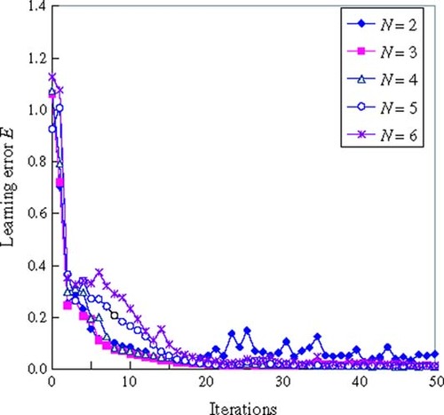
Figure 6 shows the learning error on changing the number of the delay elements of the FIR-type NN. When the number N of the delay element is 3, the learning error approaches the convergence state without any fluctuation.

Figure 6. Learning error on changing the number of delay elements of the FIR-type NN.

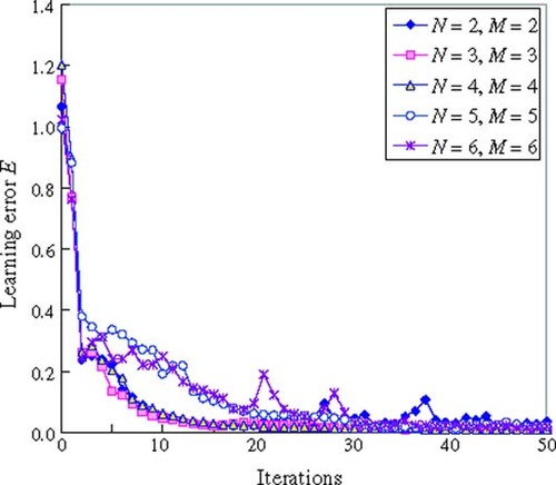
Figure 7 shows the learning error with the same number of the delay elements in the input–output side of IIR-type NN. Comparing the result (case N = 3) in figure 6 with the result (case N = M = 3) in figure 7, the learning error of the IIR-type NN approaches convergence faster than the FIR-type NN. This can be observed, for example, at iterations 10.

Figure 7. Learning error on changing the number of delay elements of the IIR-type NN.

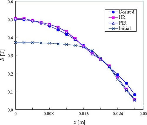
Figure 8 shows comparisons of the magnetic flux density distribution using two NNs between A–B in the shape optimization. The differences in the magnetic flux density distribution after the optimization approaches a very small value irrespective of the learning processes of the network. However, in case of the FF-type NN, the learning number was found to be 748, which is larger than those of the FIR-type and IIR-type NNs.

Figure 8. Magnetic flux density distribution between A–B in the shape optimization (comparison of the IIR-type and FIR-type NNs).

Figure 9 shows comparison of the learning error in the FIR-type and the FF-type NNs, and figure 10 shows the comparison of the learning error of the IIR-type and the FF-type NNs. We can admit that the learning error decreases faster in both cases of FIR-type and IIR-type NNs than in the FF-type NN, where the learning error fluctuates slightly in the iteration process.

Figure 9. Comparison of the learning error of the FIR-type and the FF-type NNs.

Figure 10. Comparison of the learning error of the IIR-type and the FF-type NNs.

Figure 11 shows the comparison of the learning error of the IIR-type and the FIR-type NNs. We can notice that the IIR-type NN converges faster than the FIR-type NN.

Figure 11. Comparison of the learning error of the IIR-type and the FIR-type NNs.

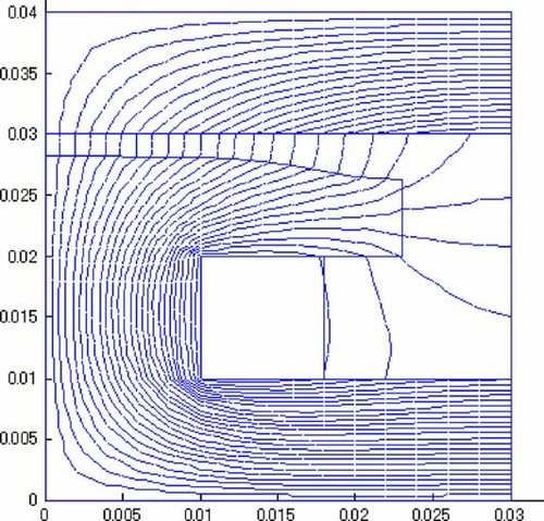
Figure 12 depicts the shape and the magnetic flux distribution with the IIR-type NN after the optimizations were attained, and a good agreement was seen with the other two networks. This result shows that the calculation with the NNs is appropriate.

Figure 12. Shape and magnetic flux distribution after the optimization.

5. Conclusions

The architectures and the learning algorithm of a FIR-type and an IIR-type NNs, which were proposed by the authors, were presented and applied to a magnetic pole shape optimization problem. These NNs are capable of reducing the learning iteration in comparison with the conventional FF-type NN, and of stabilizing the learning process. Particularly, in the case of the IIR-type NN, the learning iteration and error are the smallest of the three types of NNs. As a result, the IIR-type NN was proven to be useful for the problem that takes learning iterations long and needs stabilization of calculation, such as the optimization problem.