Abstract
The article examines stable identification error behaviour over variations of initial data. Both initial–boundary temperatures and internal temperature measurement schemes are the design objectives to reconstruct thermal properties with minimal errors. It is proved that the behavior of identification error is completely expressed by two groups of dimensionless factors. The method developed also reveals the singularities of thermal properties estimation. New conditions of violation of the inverse problem solution are deduced. The results obtained depict generic cases of the identification error distribution over a specimen length during initial data variations, when the solution satisfies conditions of inverse problem regularization.
1. Introduction
The substantiation of the computerized inversion is commonly performed in terms of numerical stability. The theory of ill-posed problems Citation1–3 investigates a noise effect on a solution error. Of course, a noise level is a parent of identification errors. To reduce their values after the solution stabilization optimal sensor locations are designed. However, the precision of a stable inverse problem solution with noisy data depends on set of all initial information, and identification errors are not only a function of noise level but also sensor locations. Therefore, the investigation of error behaviour should envelop all initial data including various combinations between initial and boundary functions of a direct problem studied. Here the restriction of arbitrary variations of ill-posed problem solution is considered as a solved problem. The stress is laid on further identification error reduction when the commonly known regularization conditions are satisfied. From a practical viewpoint, the shortcoming of the present theory of the experimental design, considering the optimal design without respect to impact actions, should be eliminated. Overall, the stable error behaviour will be described covering its dependence over both a noise level usually examined in the theory of ill-posed problems and measurement schemes studied in the theory of experimental design.
The above formulation puts new theoretical questions. What is a full set of factors that ensures a reduction of stable identification errors with a fixed noise level? More generally, do criteria exist completely defining the solution error behaviour for every inverse problem having an individual structure of diminishing factors, which differ among themselves, even within the framework of one kind of a mathematical model of a problem?
We offer to seek all the factors that depict the stable identification error behaviour far and wide. Taking into account that in a given class of problems the sought measurement scheme depends on identified and unknown properties, the determination of the solution structure of the experimental design problem will allow us to establish the essence of a local optimality in the strongly nonlinear case of a state function dependence on desired properties. Besides, it is important to grade these factors according to their effect on the identification precision as well as to elicit the worst and best conditions of the inverse problem formulation.
In contrast to the present theory of the experimental design with inverse problems Citation4–13, we develop the idea of explicit determination of so-called guaranteed identification error and propose the technique to study its stable behaviour during initial data variations Citation14. The final purpose is the guaranteed determination of most informative measurements and best external impacts in the framework of the action of worst measurement conditions. Additionally, the complete picture of identification regularities is aimed as one of a main drive. In the issue, the numerical approach is developed to substantiate the inverse problem formulation. This is possible due to the studying of the stable identification error behaviour that mirrors all the basic regularities including the conditions of the solution absence, its nonuniqueness and optimal identification.
Being formulated on the idea Citation14, the present article initiates the heat process investigations to elicit the typical best and worst conditions of thermal property estimation. Here the stress is laid on the analytical study to understand the experimental design regularities. Due to the explicit form of observation matching equations, we reveal the fundamental group of dimensionless factors that determine the stable behaviour of the identification error. The next article shall represent the technique implementation for the optimal identification of boundary parameters and model coefficients simultaneously to study the regularities of the estimation as much as possible the unknown test object properties. Further, the estimation of nonlinear thermal properties will be investigated. Above series of investigations are convenient to evaluate the new optimal design features that are unknown at present.
The article is organized as follows. In section 2, a brief description of the technique offered is given. The new design tests are introduced to determine the sense of the sought solution. Section 3 is devoted to the optimal estimation of constant thermal properties. The analytical solution allows us to respond to the main question of the investigation and educes the structure of factors to ensure the identification error reduction. Being formulated on these factors, the solution of the design problem is obtained. In section 4 the technique is also used to analyse the identifiability violation. The new peculiarities of inverse problems are revealed. Their detection argues that the analytical study of the linear models indicates important features of inverse problems.
2. Guaranteed identification errors
Let us give a brief description of the technique that deals with the optimal experimental design in the sense of guaranteed errors. All necessary details of the approach formulation are discussed in Citation14,Citation15. In this section, we pay attention to the idea with respect to the problem studied below.
2.1. Problem formulation
Consider a test object with a state function u(x, t) in spatial domain Q and time interval (0,T) satisfying the well-posed direct problem
where La denotes the adequate model of the object studied, a =
is the vector-function of unknown object properties, f is the external impacts. Existence of a unique element u for given a and f are assumed. The kind of operator La and functional properties of unknown quantities a in the framework of the present investigation will be stated in section 3. Other models were considered in Citation14,Citation15.
It is also supposed that a sample
burned with a noise ϵ,
deviates from its prototype by a known amount
on each statistically independent ith group of the observation. The prototype function
is the direct problem solution with the actual value
of test object properties. Their magnitudes are considered to be unknown. The quantity δi is the commonly known estimator of the ith sensor measurement errors,
. The latter does not require any hypothesis to the error distribution function as well as the expected value and covariance matrices are not specified. The measurement error estimator is the upper bound of the noise through the article. This may be derived at every experiment.
It is required to seek both the optimal measurement scheme
and external impacts guaranteeing the reconstruction of desired properties
with the minimal identification error
. The number of sensors m and sampling times n are coordinated with the number of unknown parameters p and are defined according to the condition supporting the admissible minimum of measurements Citation16. The sample with minimal volume of measurements, m × n = p, is one of the objectives of the present investigation. In this case, the matching with the sample should be formulated as the equality.
2.2. Design tests
Essential features of the technique offered are the type and character of the design problem solution. They are based on the explicit form of the identification error generated by the worst measurement conditions.
Definition 1
A guaranteed identification error is a minimal value of the worst accuracy of a stable sought quantity reconstruction obtained among all possible variants of the action of the maximum admissible error at each observation.
The idea suggests the examining of not every inverse problem solution, but only those which satisfy the conditions of sufficient stabilization. Among all relevant stable solutions it is necessary to minimize the one with the worst identification error. This specifies substantially the concept of the experimental design with ill-posed problems, because a method without regularization gives rise to uncertainty in the further design problem solution.
Also, the notion implies the noise model as the upper bound of measurement errors. A similar model conveys a wide class of noise sources and allows one to analyse many practically important cases. One of them is a sample with a small volume, for which the traditional statistics cannot be applied. In this case the matching with a sample should indicate 2p variants of the measurement error action.
As is noted, we consider only the stable behaviour of the problem solution. This means that the experimental design should satisfy the conditions of the inverse problem regularization. Consequently, the approach is developed to study the errors when the identification is provided for the restriction of a domain of admissible solutions and is coordinated with accuracy of measurements.
It should be emphasized here that the idea developed is based on two requirements of solution regularization. One of them is a restriction of a domain of admissible solutions. The other is a matching of the inverse problem solution with noisy data separately at each sample. A computerized inversion, without the sufficient restriction results in large errors despite a stability of obtained solutions. Similarly, a poor matching causes large identification errors even with sufficient restrictions. If the identification method does not ensure both the necessary matching and sufficient restriction, then it is impossible to derive the satisfactory estimation since specific, as a rule, small noise level. Choice of a relevant stabilizer and matching norm guarantees the precision of the inverse problem solution even with intense measurement noise Citation17, Citation18. Formulation (1–3) satisfies the above conditions. Therefore, Definition 1 deals with the conditions of the optimal identification including the requirement of sufficient solution regularization.
In addition, taking the existence of the nonunique roots of the observation matching equations into account, it is important that the offered approach formulates a stabilizer minimization. The latter ensures the necessary filtration of roots closing the question of the unique identification. Next it will be demonstrated how this rule improves the solution precision even in the case of the constant sought quantities when a domain of admissible solutions is not expended. Other idea advantages concerning the existence of inverse problem solutions, which cannot be derived in the framework of the conventional approaches, are discussed in section 4.
Thus, the optimal solution obtained in the framework of Definition 1 is the minimized identification error under the worst observation conditions, when all regularities of inverse problems are taken into account.
To specify the experimental design test, in terms of the guaranteed identification error, we introduce the following criterion.
Definition 2
R-optimal observation design is a measurement scheme that minimizes a root mean square norm of guaranteed identification error.
In this case the desired test is , where υk denotes the absolute identification error of the quantity ak. The sought optimal measurement scheme Ξ(R) should minimize the rms-error,
, and the value υ(R)=
is the R-optimal guaranteed error.
In addition to the rms-estimator, other error norms of the inverse problem solution can be considered. In particular, it is the absolute-error estimator.
Definition 3
M-optimal observation design is a measurement scheme that minimizes an absolute norm of guaranteed identification error.
In this case the estimator is used. Consequently, the min-max solution
is the essential of the M-optimal design and the value
is the M-optimal guaranteed error.
The criteria introduced are the typical error estimators in the theory of approximation. However, they differ from the conventional design tests Citation4,Citation5. The basic difference is the transition from the implicit to the explicit form of the identification error. Other differences are regarded with the model of measurement errors. The postulation of a noise distribution and their covariance matrixes are not required. The sufficient volume of statistical information for the existence of the design problem solution is a limited norm of noise, , where
denotes the admissible bound of the noise that will be introduced in subsection 4.2. Thereby, the optimal experimental conditions are derived with the most general assumptions on the noise, including fixed errors. In the mean time, additional information including a noise distribution law may be used to increase the estimation precision.
2.3. Planning procedure for constant desired quantities
Following Citation14 the experimental design problem is divided into four subproblems. Generally, they consist in a minimization of a stabilizing functional on a set whose elements differ from actual sought quantities at most by fixed value, which should satisfy the observation matching equations. The idea is based upon the regularization scheme, which was offered in Citation19. Its main advantage is the absence of the regularization parameter. This is attained due to a direct minimization of a stabilizing functional.
If the sought quantities belong to the Euclidean space, then the above-mentioned subproblems are formulated as follows. The first one is the minimization of the function
(------117094--1)
with the restrictions
(------117094--2)
where Ω denotes the stabilizing functional Citation1, υk is the absolute identification error of the kth quantity ak. The second subproblem is a direct problem with the preset initial–boundary conditions and current magnitudes a(υ) satisfying the preceding subproblem. Its solution
determines the state function concerning the current value
. The third one is the determination of the identification error υ from the equations conveying the model state matching with the sample:
(------117094--3)
Below, these equations are determined as observation matching equations. Their solutions give the identification errors
. Finally, the fourth subproblem is the minimization of the function υ with respect to the variables of Ξ.
Formulation Citation1–3 is posed for the constant sought quantities studied below. More general functional dependencies including temperature-dependent thermal properties can also be considered. The idea remains without a change and identification errors should satisfy the observation matching equations together with a minimization of a stabilizing functional. Relevant stabilizers Ω for the variable sought quantities are taken in conformity with the recommendations Citation17, Citation18.
Summarizing, we note that the solution obtained below is only one of the possible applications of the guaranteed error approach Citation14. By virtue of its generality, no limitations are imposed on the mathematical models used. Further generalizations, both on the kinds of boundary conditions and sought quantities as well as the choice of other measurement scheme and test criteria, may be accomplished after the studying of basic experimental design regularities. In particular, other measurement schemes and boundary conditions of the second and third kinds will be discussed in the next article. The present investigation aims at proving the existence of the experimental design problem solution structure to understand the background of further complex mathematical model examination.
3. Estimation of constant model coefficients
Let us consider the typical thermal models being formulated on the approach described in the previous section. Simple cases with constant coefficients will be studied first because the effect of initial–boundary temperatures on the identification error behaviour is not investigated at all. The models with temperature-dependent properties are expedient for the studying after the examination of initial data effect.
3.1. Mathematical model
Let us specify the following mathematical model
(------117094--4)
It is required to seek such Ξ = {xi, ti}i = 1,2, for which the known internal measurements
identify the coefficients {ak > 0}k = 1,2 with the minimal guaranteed error on the Euclidean
or absolute
norms. The measurement schemes determined to the above test μ(R) and μ(M) are termed as R- and M-optimal. Here
denotes the relative identification error, the coefficients
regard with the actual state
, ϵ is the measurement noise, δi denotes the upper noise bound of the ith sample. The sample volume is selected under the condition to support its admissible minimum, m × n = p. On this basis we consider only the one sampling time (n = 1) for each of two sensors (m = 2).
To reveal analytically the sought features of the optimal identification, a number of premises are accepted. We deal with the constant coefficients a1,a2= const>0. A specimen density is considered as a known constant in the coefficient a1. Also, the external impacts are limited to the quantities f, u0, v1, v2 = const. These restrictions simplify the analysis of the optimal identification over the initial data. In addition, the above simplification does not reduce the number of ratios between the external impacts that establish the existence of the typical cases of the identification error behaviour. They envelop many practical cases, as well as the characteristic ratios between the initial and boundary temperatures. As one can see below, the latter ratios determine the extensive set of the stable identification error behaviour.
Note that the approach developed does not require the additional compatibility conditions of the inverse problem solutions except for the above-mentioned conditions relatively to the sought properties and impacts. The conditions of the absence and nonuniqueness of the inverse problem solution are the objectives of the present study and are revealed in section 4 with the help of the approach developed.
The procedures described in subsection 2.3 are realized for model (4) as follows. First, the solution of the minimization subproblem has been sought
. Second, the state function of the test object has been determined
Third, substituting above solution u(x, t) into equation (3) and using the measurement model yields
where
Finally, passing to the guaranteed error and attracting the maximal measurement error, we obtain the following observation matching equations
(------117094--5)
These two equations indicate the worst conditions of the approximation of the sample uδ by the state function
. They set the error corridor ±δ respectively to the noisy data. The passing to the difference between the true state
and guaranteed solution
gives other corridor, namely ±2δ. The change of the corridor width is caused due to the consideration of the worst measurements.
The solution of equation (5) for the fixed δ determines the relative identification errors μkk=1, 2. The absolute norm in (5) generates four cases of the state function matching with the sample
. Consequently, four variants of equation (5) should be solved for each sensor location and sampling time. According to Definition 1 the guaranteed identification error is the solution with the minimal norm. This solution should be minimized respectively to the variables x and t.
3.2. Optimal sensor locations
Let us study the general regularities of the behaviour of functions {μk(x, t)}k=1, 2 during the variations of their independent variables. The qualitative analysis of the solution features will be involved to elicit the optimal experimental conditions. We will reduce the determination of the maximal or minimal errors to the study of cases, when the functions {Fl}l=1, 2, 3 or their terms are zeroing or maximizing.
To start being based upon the kind of {Fl}l=1, 2, 3, we reveal the necessary condition of the restriction of identification errors, t→∞. This condition divides the observation matching equations into two separate equations. One of them completely determines the error μ2, and the other includes μ2 as a parameter. Hence, the determination of the optimal observation design is reduced to studying primarily the behaviour of the function μ2 and next μ1.
As a result, the least guaranteed error of the thermal conductivity estimation is derived
(------117094--6)
where
. The case f = 0 has the individual kind of the latter criterion and is separately considered in subsection 3.5.
Formula (6) has been obtained by the substitution of the stationary solution of problem (4) into the observation matching equation. After the minimization of stabilizer (1), the guaranteed error (6) is educed and the first optimal sensor location is revealed,
. The result is valid for each a1,a2=const>0 and arbitrary constant {,f≠0,u0,v1,v2}.
Above criterion ℜ indicates a very important feature of mathematical models. As it seems, the basic behaviour of identification errors is expressed by the generalized factor. To emphasize the conditions that produce the major effect on the precision of the inverse problem solution, we introduce the next notion.
Definition 4
Indeterminacy power of mathematical model identification is a factor determining a level of a guaranteed error according to the preset measurement errors and to the kind and magnitude of external impacts.
The notion terms those actions applied to a specimen, which should reduce the identification errors to zero. The relevant factor expresses not only the noise level and also indicates a certain abstract driving force. Its kind is determined by the mathematical model under the study. Different mathematical models will have different kinds of the indeterminacy power factors.
Let us now analyse the behaviour of the function μ1(x, t). Its character is determined by the stage of the thermal process and magnitudes of {,f,u0,v1,v2}. The restriction of the exponential growth of functions {Fl}l=1, 2, 3 can be attained if their terms tend to zero or have a maximum during the variations of variables x and t. Below each of these cases are considered.
At the initial stage of the process, if t ∼ 0, then a sharp growth takes place since the multipliers of μ1 in the exponential terms of {Fl}l=1, 2, 3 are the linear functions over the variable t. Accordingly, the necessary restriction of the exponential term growth is attained by the choosing x such that the functions sin(2k−1)πxℓ and tend to zero. Therefore, at the initial stage of the process the identification error μ1(x, t) is decreased, when the measurements tend asymptotically to the specimen boundaries, x→0 or x→ℓ. Here, the local or global character of the error minimum is established by the ratio between the external impacts {f,u0,v1,v2} because of the effect either the even or odd terms of the series of equation (5) on the restriction of the exponential functions growth. At themselves boundaries x=0,x=ℓ, from (5) follows that the function μ1(x, t) has a discontinuity of the second kind. In the issue, the measurement schemes
(------117094--7)
are R- and M-optimal, if the condition
is satisfied and the free term f does not exceed the value that establishes in equation (5) the significance of the function F1 against F2 and F3. Identification error behaviour during the variations of the free term f will be considered in subsection 4.2.
The ratio between the initial–boundary temperatures in (7) causes the mutual compensation of the even and odd terms of F2 and F3. Therefore, the growing of μ1 is not minimized though the sensor location ensures the maximal values of the harmonics of equation (5). On this basis, if the condition u0≅v1 or u0≅v2 takes place, then the global minimum of the design test tends to one of the specimen boundaries. The existence of the optimal observation in the immediate vicinity of the specimen boundary and at the onset of the thermal process is a fact previously unreported. This inference is of doubtless interest to the design theory.
If t ≫ 0, then the variations of the parameters of exponential terms of equation (5) are insufficient to restrict the growing of μ1. The required error reduction can be attained, when the sensor location is such that the harmonics of equation (5) attain their maximum. In view of the convergence of the series of equation (5) only the first terms are significant to limit the growing of μ1. Therefore, the minimum of the design test should be attained at the domain of x = 0.25 ℓ, or x = 0.5 ℓ, or x = 0.75 ℓ. For the specific f the effect of terms of equation (5) on the restriction of the exponential functions growth is ensured by the gap between the temperatures u0 and {vk}k=1, 2. The magnitude of the gap establishes the local or global character of the design test minimum. The worst thermal loading satisfies the condition u0=(v1+v2)/2. The second optimal sampling time is determined as the locally optimal magnitude. Overall, the measurement schemes
(------117094--8)
are the R- and M-optimal, if the relevant initial–boundary ratios are set. In this case the optimal sensor location
cannot be precisely determined. Its value deviates from x = 0.25 ℓ, or x = 0.5 ℓ, or x = 0.75 ℓ with the decreasing of the thermal diffusivity a=a2/a1 because the convergence velocity of the series of equation (5) depends on this magnitude. Thereby the second optimal sensor location
should be refined during the change of the test object thermal properties. However, the optimal location of the second sensor is varied within the limits of the above defined regions. Below it will be demonstrated that the transition between the regions of the optimal sensor location occurs in steps.
Let us consider the optimal measurement scheme of controlled experiments. It is assumed that the external impacts are not fixed, and they can be modified in the desirable direction. There is a specimen loading satisfying the condition
(------117094--9)
which may be termed as the best guaranteed loading. This means that the optimal location
does not depend on the magnitudes {,f,u0,v1,v2} and is not changed during the variations of external impacts. To determine the optimal sensor location, when the boundary temperatures satisfy (9), we subtract one from other equation (5) for different x′ and x″. This yields
From it follows the condition
that indicates the reduction of μ1 relatively to the variable x. Thereafter the error μ1 has the minimum for the arbitrary {,f≠0,u0,v1,v2}, when the sensor location is selected such that the functions
have maxima. Among all the relevant values
only one of them, x=ℓ/2, ensures the required maximum at each term of equation (5). Thus, if condition (9) is satisfied, then the middle of a specimen becomes the unique point, where measurements ensure the identification of the thermal properties with minimal errors. The relevant optimal measurement scheme is defined as follows
(------117094--10)
Note that there are impacts, for which the solution of the experimental design problem does not exist. Similar cases will be considered in section 4.
The consideration of all the possible combinations of the initial data should be studied to response the complete solution of the experimental design problem for the fixed mathematical model. This can seem the extensive condition. Next it will be proved that only two groups of dimensionless factors completely signify the domain of initial data and response the relevant conditions of the solvability and optimality. In this case, all the solutions of the experimental design problem are assorted into the finite number of typical groups.
It should also be stressed that the aforesaid solutions of the optimal experimental design problem were revealed despite the essentially nonlinear dependence of the model state on desired quantities and under the assumption of the arbitrary nature of the measurement noise. Thus, even the strongly nonlinear experimental design problem admits the aggregation of its solution and has the strictly defined optimal measurement scheme. The determination of a similar solution structure points out the key direction of further investigations of complex mathematical models.
3.3. Factors of identification error reduction
The error of the inverse problem solution is reduced by some ways. As it follows from (6), one of the ways is the noise level decreasing. This commonly known fact is usually considered as a solo factor of the error reduction. The analysis of the observation matching equations reveals the novel ways.
First, formula (6) indicates the requirement of the increasing of the free term f. Moreover, there exists a magnitude , for which the identification error does not exceed the noise level
. Naturally, the inference is held, if a specimen heating does not disturb the adequacy of model (4).
Second, the gap between the initial and boundary temperatures {u0,v1,v2} diminishes the error μ1 because the multipliers in the exponential terms of equation (5) are increasing. If the boundary temperatures vk→∞,,k=1,2, then for the fixed u0 we obtain
(------117094--11)
This expression indicates that the function μ1 tends to
if the gap between the initial and boundary temperatures are unrestrictedly increasing. Therefore, the variations of v1 , v2 do not absolutely reduce the identification errors to zero.
Let us compare the significance of the reduction factors found. The most essential factor is the elevation of the free term f. It follows from the majorization of the function μ1 by the value
, which is independent on the temperatures {vk}k=1, 2. For non-uniform model (4) the gap between the initial and boundary temperatures has only a local role as a reduction factor.
Note, that there is a third factor of the error reduction. It is a sample volume. Its investigation is not the purpose of the present study of the most informative measurements based on the minimal volume of the sample. This factor is a subject of future investigations.
The operation of the indicated factors can be expressed with the generalized criteria. Let us introduce additionally to the above criterion the new dimensionless factors
. The variation of the initial data
(------117094--12)
and appropriate choice of the dimensionless time
and sensor location ξ=x/ℓ do not change the solution of equation (5). This means that the errors of the inverse problem solution are invariant regarding transformation (12).
The latter is a theoretically important fact. The introduction of the factors {ℜ,Φ1,Φ2} allows us to reveal the typical cases of the identification error behaviour. These factors establish two kinds of the observation matching equation terms. The first one does not depend on the spatial coordinate. The remaining terms depend on the spatial coordinate. The groups of terms are consequently connected with the factors ℜ and {Φ1,Φ2}. The variations of ℜ have effect on the free term of the observation matching equations. This determines the magnitude of the errors {μk(x, t)}k=1, 2 but does not change their behaviour over the specimen length. The variations of {Φ1,Φ2} change the spatially dependent terms. Consequently, they shape the error distribution over the specimen length. The conditions of their zeroing, Φ1=0, or Φ2=0, or
determine the status of the identification error distribution. These conditions have the simple physical sense. It is necessary to take into consideration that the unlimited growth of {Φ1,Φ2} does not reduce the identification error up to zero.
Thus, the factors {Φ1,Φ2} determine the kind of identification error distribution over the specimen length. The criteria, which express a shape of identification error distribution, should be determined as a special notice.
Definition 5
A form-factor of an identification error mode is a set of external impacts determining a character of an identification error distribution versus a sensor location.
The use of the dimensionless factors {ℜ,Φ1,Φ2}, regarding which the identification error is invariant, guarantees a similar error behaviour on the domain of the initial data. As a result, the generic identification error groups are revealed not as a partial case of certain numerical experiment, but as a feature of the mathematical model under study. This means that the revealed worst and best impacts, regions of error growth, locations of the minimal error, kinks and other characteristics will be similar for a wide range of initial data. In the issue, the fundamental effect of the ratio between the initial and boundary temperatures on the kind of the optimal design solution is elicited and the existence of the typical groups of the solutions is proved.
3.4. Numerical solutions of observation matching equations
Further details of the identification error behaviour are revealed numerically. indicates the typical identification error behaviour. Each curve represents the rms-error minimized on time:
The values μ1 and μ2 have been sought from equation (5). The observation matching equations have four variants of the measurement error action. Among them, for the current sensor location and sampling time, the maximal magnitude of the solutions is taken as the final identification error μrms. This worst error is minimized on time. The first sensor location x1 and sampling time t1 were fixed,
. Variations of x1 are not required because of its strictly defined optimal location in the middle of the specimen for all {ℜ,Φ1,Φ2}. The second sensor location is varied at the interval 0<x2<ℓ. The factor ℜ was fixed because of its effect only on the free term of the observation matching equations. The numbering of the curves indicates the evolution of the error distribution during the boundary temperature variations.
Let us discuss the results obtained. The main value is the structure revealing of the experimental design problem solution. Its basic features are the existence of the generic ratio between the impacts, conditions of the error growth including the cases of the violation of the identifiability and also specific regions of the minimal identification error. They all indicate the existence of the strongly defined optimal measurement schemes. The finding of these features is a valuable advantage of the offered design technique.
On the whole the solution structure of the problem studied is divided into two parts. Each of them has its own groups of the typical identification error behaviour.
The first part, , reflects the condition when Φ1>0 and the right boundary temperature v2 does not exceed the initial state u0. Each of the three cases has its own best and wrong locations of the second sensor. All of them were revealed in subsection 3.2 and they are the specimen centre, its middle region, quarter of the length and neighbourhood of the boundaries. The kinks are the consequence of the discontinuity of the sought sampling time. The ones occur due to the existence of the nonunique solution of the minimization problem. The first typical error mode takes place, when the initial and left boundary temperatures satisfy the condition Φ1≤0 (, curves 1–6). In this case the second optimal sensor location
moves from the middle of the specimen to the right boundary while the left boundary temperature v1 tends to the initial temperature u0. The change of the optimal position occurs in step. The next typical error distributions take place if
(, curves 7–10). This mode features the transition of the optimal sensor location
from the right boundary to the region of the quarter specimen length. Zero values of the form-factors generate the regions with the large but limited identification error,
. Curve 10 indicates the sharp growth of the error in the middle of a specimen. The reason for the growth is studied in subsection 4.3. The last typical error mode (, curves 11–17) indicates the appearance of the local minimum in the middle of a specimen, which is transformed to the global one in progress of the growing of the left boundary temperature, v1≫u0. According to condition (11) the value of the global minimum tends asymptotically to non-zero value of the identification error.
Figure 1. Typical groups of the identification error behaviour. The temperature v1 is varied, , the temperatures u0 and v2 are fixed,
, the small circles denote the minimal errors. The cases (a), (b), (c) indicate the conditions v2<u0 and (1) v1=0; (6) v1=u0; (10) u0=(v1+v2)/2; (17) v1≫u0. The cases (d), (e), (f) indicate the conditions v2 > u0 and (1) v1 < 0; (3) v1=0; (5) u0=(v1+v2)/2; (10) v1=u0; (13) v1≫v2.
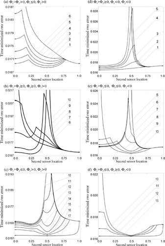
The second part of the generic error distribution, , depicts the condition Φ2 < 0, when the right boundary temperature v2 exceeds the initial state u0. Three cases of the solution groups represent the structure of the optimal design. As in the preceding cases , the transitions between the solution groups are generated by zero values of the form-factors. The differences with the case Φ2 > 0 are expressed by the second optimal sensor location at the neighbourhood of x=0.75ℓ (, curves 3–5 and , curves 6 and 7), at the left boundary (, curves 1 and 2) and in the middle of the specimen (). Curve 5 indicates the sharp growth of the error, when
. The identification error has a large but finite magnitude.
Summarizing the results obtained, note that the variations of the second optimal sensor location emphasize the importance of the obligatory account of the ratio between the initial and boundary temperatures. The present theory of the experimental design with inverse problems does not consider this ratio. All generic cases of the identification error distribution are expressed by the simple factors.
3.5. Uniform model
In the previous section it was indicated that the non-zero free term, f≠0, has the basic effect on the identification error behaviour. Now, let us consider the uniform model, f≡0, and investigate what happens if the internal heat source is absent. The examination of the above introduced indeterminacy power criterion and typical modes of identification error distribution will indicate the new singularities of the behaviour of the experimental design problem solution. In addition, the offered approach will be compared with the traditional design method Citation7,Citation20, where the identification of the thermal diffusivity has been studied.
We seek the optimal measurement scheme to estimate the thermal diffusivity
with the minimal error being based upon a single observation
If the initial and boundary temperatures are the constant values, then the observation matching equation (3) is of the following form
(------117094--13)
where
denotes the relative identification error,
is the true value. To reveal the optimal experiment conditions we will determine zero, maximal or minimal values of the equation (13) terms. This indicates the following regularities of the uniform model identification.
First, if u0≠(v1+v2)/2, then the indeterminacy power is
, otherwise
. For all v1=v2 its upper bound of the identification power is
. It follows from (13), when μ→∞,t→0. Second, the form-factors of the uniform model are
, Φ2=(u0−v2) (v1 + v2−2u0), if u0≠(v1+v2)/2, and otherwise Φ1=0,;Φ2=1. These factors divide all the set of initial–boundary temperatures on six typical groups of the identification error behaviour. To each of them there corresponds its own optimal measurement scheme that needs to be modified only in some details for all a > 0. The worst experimental conditions are
,
and
. On the other hand, the condition
or
evinces the best external impacts. The guaranteed lower bound of the sampling time is
.
In the middle of a specimen, x=ℓ/2, the impacts satisfying the condition u0=(v1+v2)/2 give rise to the large but bounded error, 1 < μ < ∞. At the same time, if v1=v2, then the sensor location in the specimen middle is the optimal position. The deviation from the location x=ℓ/2 grows with the difference between the boundary temperatures.
In contrast to the case f≠0, the uniform model has not the optimal locations at the neighbourhood of the point x=0.25ℓ or x=0.75ℓ. For all impacts the sensor location tends asymptotically to the specimen boundaries. The neighbourhoods of the boundaries are the optimal location for a wide range of the initial–boundary temperatures (Φ1≥0).
All the typical groups of the stable identification error behaviour for are shown in . The case
is studied similarly. Also, there are three regions of the optimal sensor location, namely, the neighbourhood of the specimen boundaries and its middle part. It is practically important that due to the boundary temperature variations the optimal measurements can be executed in the most accessible region.
Figure 2. Typical identification error distribution. The temperature v1 is varied, , the temperatures u0 and v2 are fixed, u0 > v2 , the small circles denote the minimal errors. (1) v1≪v2; (2) u0=(v1+v2)/2; (3) u0 < (v1 + v2)/2; (4) v1=u0; (5) v1 > u0 ; (6) v1=v2; (7) v1≫v2.
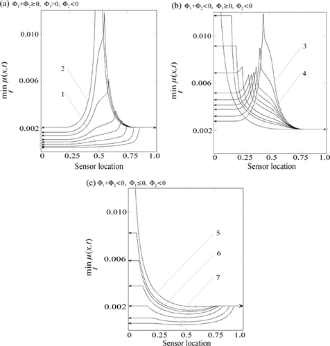
Note that the above regularities were not obtained by the traditional design method Citation7,Citation21. Our approach depicts the full regularities of the experimental design and reveals the solution structure of the design problem.
3.6. Basic features of the optimal identification
The investigation of model (4) has detected the following regularities of the simultaneous identification of the constant thermal properties. The optimal observation design is conveyed by the strictly defined scheme of measurements of specimen temperature field. The specification of non-zero free term, two boundary and two interior temperatures with one sampling time at each sensor is one of the possible experimental conditions to identify the constant specific heat and thermal conductivity simultaneously. In this case, there are six typical cases of the identification error behaviour. A noise level does not determine the mode of the error distribution, but mainly defines its magnitude.
The first optimal interior observation does not depend on the character of external impacts and sought properties. The sensor should be located in the middle of a specimen. The relevant optimal sampling time is the observation of the specimen steady state. The second optimal interior observation is localized at one among five limited regions. The optimality of each of them is determined by the ratio between the initial and boundary temperatures.
There is a wide range of the initial–boundary temperatures, when the location of the second interior observation is optimal only at one of specimen boundaries, and the best sampling time is determined at the onset of the heat process. Similar experiments feature the low gap between the initial and boundary temperatures or absence of the heat source.
The second sensor location is optimal also at the neighbourhoods of the locations {0.25 ℓ; 0.5 ℓ; 0.75 ℓ}. The first and third regions are optimal, if the initial temperature is approximately equal to the average value of the boundary temperatures and the heat source is non-zero. The magnitudes of specimen thermal diffusivity and gap between the initial–boundary temperatures determine the deviation of a sensor location. For these locations the optimal measurement time is derived only as a locally optimal estimator.
The requirement of the boundary temperatures equality among themselves is an important condition for the decrease of measurement volume. In this case, the sufficient sensor number for the estimation of model (4) parameters is defined only by one interior point (not counting the observation for the deriving of the boundary conditions).
The trait of the inverse problem solution is the existence of the indeterminacy power of the model identification. The relative criterion is determined as a ratio of a noise level to a certain abstract driving force. The upper bound of this criterion determines the existence of the inverse problem solution. Other trait groups of factors are the so-called form-factors. They indicate the effect of the initial and boundary temperatures on the error behaviour. Namely, these factors determine the kind of identification error distribution over the specimen length. However, the form-factors do not release the global tendency of the identification error to zero.
The major factors of precision improvement of the simultaneous specific heat and thermal conductivity identification are the elevation of the internal heat source strength and magnification of the gap between the initial and boundary temperatures. Among two called factors, the first one is of greater importance. For every fixed noise level, the critical value of a free term can be indicated, which guarantees that the identification error will be always a less noise level. The boundless magnification of the gap does not reduce the identification error to zero, if the free term is of non-zero value. For similar cases the identification error of the specific heat coefficient tends asymptotically to the guaranteed error of the thermal conductivity estimation.
4. Peculiarities of the inverse problem formulation
The above results completely define the choice of optimal measurements. However, there are singular cases that give rise to the degeneracy of the inverse problem solution. The analysis of the observation matching equations responses conditions of the existence and uniqueness of the solution and indicates a number of new singularities of the inverse problem formulation.
4.1. Identifiability violation
The uniqueness of the solution of equation (5) requires a sampling that does not lead to a linear dependence of the terms of the observation matching equations at the points . A linear dependence takes place, if the condition
(------117094--14)
is satisfied. From it follows that the model (4) coefficients are unidentifiable on the observation
, if and only if the measurements are done at any two locations
such that
and are executed at the same moment, t1=t2 .
For model (4) the existence of unidentifiable coefficients on a whole state was shown earlier in Citation21, where the violation of the one-to-one correspondence between the desired quantities and model state at each point of the observation domain was revealed and studied. Condition (14) specifies the violation of the identifiability, when the one-to-one correspondence breaks down at the separate points
of the observation domain Q.
We specially underline that the measurement conditions indicated above give rise to the inverse problem solution only accurate within a certain parametric set, even if the noise is absent (δ=0) and the mathematical model is heterogeneous (f≠0). For model (4) any symmetrical arrangement of measurements contains the unidentifiable observation
. The use of a similar sample leads to the complete indeterminacy of the sought properties reconstruction.
4.2. Threshold noise level
Let us consider the asymptotic behaviour for μ1→1. Using the majorizing series for t < ∞, the observation matching equation is reduced as follows:
(------117094--15)
where
, denote the certain parameters. From it follows, that for every {f≠0,,u0,v1,v2} and fixed sensor location there is a value
, for which
signifies the violation of the domain of admissible values of equation (5). Therefore, the initial data satisfying (15) generate a special case of unidentifiable observation that takes place since a certain value of a noise level
.
Condition (15) can be considered in terms of the existence of such a value
, below which (
) the satisfactory identification is impossible for any δ≠0. We offer to denote the observation condition that causes a loss of the identifiability due to exceeding of some noise level as a threshold condition.
So, if the measurement noise action is regarded, then a new aspect of the absence and nonuniqueness solution should be considered and relevant initial data must be revealed. We especially stress that the above case differs from the numerical instability. The δ-unidentifiability establishes the maximum measurement noise level guaranteeing the informative interpretation of a given sample without reference to a numerical inversion. The numerical instability conveys functional features of an inverse operator that amplify the noise effect. The results obtained show the existence of a sufficient range of the noise level that can guarantee the identification precision, if the stabilizing functional and correct observation matching are the basis of numerical inversion.
4.3. Self-compensation loading and singular sample
Let us consider the case, when the threshold noise tends to zero. Now we analyse the external impacts that give rise to the threshold conditions not for the fixed, but for every noise level.
From (15) follows that there exists a magnitude f = F * for every δ, for which the error μ1 has a large but finite value. The magnitude specifies the case, when the sum of the negative terms of F1 has the same order as the sum of the positive terms F2/(F3=0). The substantial growth of exponential terms of equation (5) is caused because of the self-compensation of loading factors {,f, u0,v1,v2}. If δ=0 and x=ℓ/2, then the estimate is
.
The external impacts responsible for the loss of identification precision owing to the self-compensation of the free term f and initial–boundary temperatures {u0,v1,v2} should be regarded as an important experimental design feature. We offer to term similar conditions as a self-compensating loading. Their existence means that there is not a monotone decreasing of the minimum of identification errors during the sequential growing of the value f.
A special case takes place when δ≠0,,x=ℓ/2 and u0=(v1+v2)/2. Being based on these conditions, the observation matching equation is transformed to the expression
For t < ∞ from latter expression follows the identification error
, where
is the time-dependent parameter. In this case the self-compensation takes place for every f≠0 and v1≠v2, i.e.
, (, curves 10b and 5d). If v1=v2, then the self-compensation is absent, because of F * = 0.
Thus, for each non-zero value δ,f,a1,a2 , and v1≠v2 it is impossible to guarantee the optimal identification of the coefficient a1, if the second measurement is done at the middle of a specimen and the initial–boundary temperatures satisfy u0=(v1 + v2)/2. For similar conditions and f≠0 the second optimal sensor location is the neighbourhood of x=0.25ℓ or x=0.75ℓ. Among them the optimal measurement is determined by the ratio between the initial–boundary temperatures. For the uniform model, f=0, the optimal sensor location tends to the specimen boundaries. We offer to term the measurement as a singular sample that gives rise to the sharp increasing of the identification error due to the self-compensation of the initial–boundary conditions at a certain sensor location for the every noise level and arbitrary free term.
Summarizing the results obtained, let us make the emphasis on the new singularities of the inverse problem formulation. There exists a threshold noise of measurements and self-compensation of external impacts. A threshold noise conveys the upper bound of the admissible observation noise. The inverse problem solution does not exist, if the measurement errors become more than the threshold level. A self-compensation loading represents a significant worsening of the identification precision because of a counteraction between external impacts. All these cases do not guarantee the satisfactory accuracy of the inverse problem solution.
Also, there exist δ-unidentifiable and singular samples. A δ-unidentifiable sample causes a loss of the identifiability due to the degeneration of the state function approximation at a certain sensor location for the fixed non-zero noise level. A singular sample conveys the observation with the sensor location and initial–boundary data, for which the sharp growth of the identification error is occurring for arbitrary external impacts at every noise level.
5. Conclusions
The solution of the experimental design problem has a strongly defined structure despite the dependence of optimal sensor locations and sampling times over the test object properties. It permits to seek the generic groups of the optimal measurement scheme as a feature of a mathematical model studied. The determination of a similar structure has the key significance to solve the design problem.
The complete solution of the experimental design problem has to envelop several directions. The revealing of the optimal external impacts, sensor locations and sampling times are the main objectives of the design. The effect of external impacts on the design test can be described as the generalized dimensionless factors. The latter is divided into two groups. One of them provides the absolute reduction of identification error to zero and others ensure the decreasing of identification error only to a certain non-zero value.
Statistical uncertainties have effect on the existence of the inverse problem solution and give rise to the violation of the mathematical model identifiability. The results obtained refine the cases of violations. Threshold noise level, self-compensation loading and singular sample are the novel aspects of the noise action.
The investigation indicates that the optimal identification can ensure a suitable precision even with an intense measurement noise and small volume of a sample. The relevant numerical method should satisfy the conditions of the stabilizer minimization and observation matching separately on each sample. The next article shall be devoted to the estimation, as much as possible, of the unknown quantities with a minimal number of sensors.
| Nomenclature | ||
| a | = | =vector-function of unknown properties |
| = | =actual properties | |
| a1 | = | =specific heat coefficient |
| a2 | = | =thermal conductivity coefficient |
| f | = | =volumetric heat sources |
| ℓ | = | =specimen length |
| p | = | =number of unknowns |
| t | = | =time |
| topt | = | =optimal time of measurements |
| u | = | =temperature field |
| = | =prototype state | |
| uδ | = | =sample |
| u0 | = | =initial temperature |
| v1, v2 | = | =boundary temperatures |
| x | = | =spatial variable |
| x(opt) | = | =optimal sensor location |
| x * | = | =singular sensor location |
| ℜ | = | =indeterminacy power of identification |
| Q | = | =spatial domain |
| Greek symbols | ||
| δ | = | =upper bound on measurement noise |
| ϵ | = | =measurement noise |
| μ | = | =relative identification error |
| μ(M) | = | =M-optimal guaranteed error |
| μ(R) | = | =R-optimal guaranteed error |
| μrms | = | =root-mean-square error |
| τ | = | =dimensionless time |
| υ | = | =absolute identification error |
| ξ | = | =dimensionless length |
| Φ | = | =form-factor of identification error mode |
| Ξ | = | =measurement scheme |
| Ω | = | =stabilizer |
Acknowledgment
The author thanks the referee for useful comments that helped to present the obtained results with greater perfection.
References
- Tikhonov, AN, and Arsenin, VYa, 1977. Solutions of Ill-posed Problems. New York: Halsted Press; 1977.
- Morozov, VA, 1984. Methods for Solving Incorrectly Posed Problems. New York: Springer-Verlag; 1984.
- Engl, HW, and Groetsch, CW, 1987. Inverse and Ill-posed Problems. Orlando: Academic Press; 1987.
- Silvey, SD, 1980. Optimal Design. An Introduction to the Theory for Parameter Estimation. London: Chapman and Hall; 1980.
- Pukelsheim, F, 1993. Optimal Design of Experiments. New York: J. Wiley & Sons, Inc.; 1993.
- Fedorov, VV, and Hackl, P, 1997. Model-oriented Design of Experiments. New York: Springer-Verlag; 1997.
- Uspenskii, AB, and Fedorov, VV, 1974. Experiment planning in inverse problems of mathematical physics, Kibernetika 4 (1974), pp. 123–128.
- Kuszta, B, and Sinha, NK, 1978. Design of optimal input signals for the identification of distributed parameter systems, International Journal of Systematic Science 9 (1978), pp. 1–7.
- Artyukhin, EA, and Okhapkin, AS, 1984. Parametric analysis of the accuracy of solution of a nonlinear inverse problem of recovering the thermal conductivity of a composite material, J. Eng. Phys. Thermophys. 45 (1984), pp. 1275–1281.
- Sun, NZ, and Yen, WG, 1990. Coupled inverse problems in groundwater modeling. Identifiability and experimental design, Water Resources Research 26 (1990), pp. 2527–2540.
- Taktak, R, Beck, JV, and Scott, E, 1993. Optimal experimental design for estimating thermal properties of composite materials, International Journal of Heat Mass Transfer 36 (1993), pp. 2977–2986.
- Emery, AF, and Nenarokomov, AV, 1998. Optimal experimental design, Meas. Sci. Technol. 9 (1998), pp. 864–876.
- Dowding, KJ, and Blackwell, BF, 2000. "Design of experiments to estimate temperature dependent thermal properties". In: Inverse Problem in Engineering. Theory and Practice. New York: ASME; 2000. pp. 509–518.
- Romanovskii, MR, 1990. Planning an experiment for mathematical model identification, J. Eng. Phys. Thermophys. 58 (1990), pp. 1018–1026.
- Romanovskii, MR, 1993. Experimental design method with general assumptions about the form of the model of the experimental object, Industrial Laboratory 59 (1993), pp. 89–96.
- Romanovskii, MR, 1989. Mathematical modeling of experiments with the help of inverse problems, J. Eng. Phys. Thermophys. 57 (1989), pp. 1112–1117, (Consultants Bureau, New York, USA).
- Romanovskii, MR, 1982. Inverse problem regularization under the scheme of separate matching with observation, J. Eng. Phys. Thermophys. 42 (1982), pp. 110–117.
- Romanovskii, MR, 1983. Investigation of regularization of heat-exchange parameters estimation, J. Eng. Phys. Thermophys. 44 (1983), pp. 801–809.
- Romanovskii, MR, 1980. Regularization of inverse problems, High Temperature 18 (1980), pp. 135–140.
- Alifanov, OM, Artyukhin, EA, and Rumyantsev, SV, 1995. Extreme Methods for Solving Ill-posed Problems with Applications to Inverse Problems. Wallinford, UK: Begell House, ; 1995.
- Romanovkii, MR, 1982. Uniqueness of the solution of the inverse problem for the coefficients of the linear heat conduction equation, J. Eng. Phys. Thermophys. 42 (1982), pp. 351–357.