The adjoint method coupled with the modal identification method for nonlinear model reduction

Abstract

In order to obtain reduced models (RMs) from original detailed ones, the Modal Identification Method (MIM) has been developed for several years for linear and then for nonlinear systems. This identification is performed through the resolution of an inverse problem of parameter estimation. So far, the MIM was used with the Finite Difference Method (FDM) for the computation of the gradient of the functional to be minimized. This leads to important computation times. In order to save it up, the Adjoint Method (AM) has been coupled with the MIM to compute the gradient. All the equations related to the reduced model, the adjoint equations, the gradient and the optimization algorithm are clearly expressed. A test case involving a 3D nonlinear transient heat conduction problem is proposed. The accuracy of the identified RM is shown and the comparison between the proposed AM and the classical FDM shows the drastic reduction of computation time.

Keywords:

• Reduced Model
• Modal Identification Method
• Inverse Heat Conduction Problem
• Adjoint Methods

1. Introduction

Multidimensional nonlinear Inverse Heat Conduction Problems (IHCPs) usually involve the use of a high order detailed model related to the space discretization. Due to the large number of degrees of freedom of the systems, the optimization algorithms used to solve the IHCP may be tremendously time-consuming. This drawback leads us to identify some models that have a much lower number of degrees of freedom. Starting from a Detailed Model (DM) of the system, the Modal Identification Method (MIM) is applied to build the corresponding Reduced Model (RM). The use of such RM allows important reductions of computation time when solving either direct or inverse problems 1,2. Although RM is built once for all, the computation time needed to obtain it increases with the number of parameters to be identified and especially with the nonlinearities.

So far, the identification of reduced models through the MIM has been based on gradient algorithms coupled with the well-known forward Finite Difference Method (FDM). The objective function to be minimized is the mean-squared discrepancy between the outputs of the reduced model and of the detailed model. When the direct detailed model is nonlinear, the number of iterations needed to identify the reduced models may be large leading to a high time-consumption. Moreover, the FDM needs, at each iteration of the optimization algorithm, (m + 1) full nonlinear resolutions of the models to evaluate the m components of the reduced model. Added to this great drawback, the FDM only gives approximations of the functional gradient thus yielding to even more computation time. In order to save-up some computation time when building the RM, we have coupled the optimization algorithm with the Adjoint Method (AM). The corresponding lagrangian penalizes the reduced space and time-dependent state representation as well as the output system. The resulting adjoint problem involves at most two more linear systems. The gradient of the functional resides in the end in a single matrix–vector product. The numerical tests presented in the article prove the ability of the adjoint methods to identify reduced models and show the drastic reduction of computation time needed to identify the reduced models.

The article is organized as follows. In section 2 we state the DM of concern. This DM deals with a three-dimensional nonlinear mixed-boundary transient diffusive problem with selected outputs. We then state the RM structure derived from the structure of the DM while complying with all the nonlinearities taken into account. In section 3, the identification of the components of the reduced model is formulated as an optimization problem. For efficiency considerations, the optimization problem is based on a lagrangian formulation. The corresponding adjoint problem along with the objective function gradient and the global optimization algorithm are theoretically written down. Section 4 is then dedicated to the numerical results. This section first shows that the AM coupled with the MIM is very efficient for RM identification. As a second part, this section shows the high reduction of computation time when using the adjoint theory when compared to using the classical FDM. Then, this section shows a validation of the identified RM. Eventually, section 5 is dedicated to conclusions and extensions of the presented work.

2. The nonlinear diffusion model

2.1. The detailed model formulation

Let us consider that the continuous physical phenomenon of concern is a priori governed by the parabolic unsteady diffusive evolution equation (1) in (x, t)∈Ω×I where x∈Ω⊂ℜ³ and t∈I=(0, t_f): Find ϕ = ϕ(x, t) such that: (------120570--1) where α is the inertial coefficient, β is the diffusion coefficient, ∇ is the vector differential operator, n is the outward unit normal vector, ϕ = ∂ϕ/∂t where t is the marching variable, and where ∂Ω₁∪∂Ω₂ is a partition of the border of Ω. The strong direct problem is in most cases nonlinear in the sense that coefficients α and β, as well as the functions f and h, may depend on the state variable ϕ. For instance, it will be seen in this article that β is considered as a linear function of the state variable. Moreover, numerical results presented in section 4 consider the convective-type Neumann condition of the form on one part of ∂Ω₂ while a prescribed flux density is applied on the other part of ∂Ω₂. The direct detailed problem being complex (three-dimensional and nonlinear), there is no analytical solution for the state variable ϕ. As for most parabolic problems, the continuous partial differential equations involved in the direct model equation (1) have to be approximated twice. One step of approximation concerns the space. The other one concerns the marching integration. The order in which approximations are performed is not fundamental. We present here the case where the state variable is first space-approximated. Using, either the finite element method 3, the finite difference method, the meshless method 4, or the finite volume method 5, etc. the continuous partial differential equations (1) are replaced by the time-dependent matrix system of order N given in equation (2): Find Φ=Φ(t)∈ℜ^N such that: (------120570--2) where the matrix may depend on the state Φ and the dimension N is related to the size of the space discretization 6. Moreover, U is the explicitly expressed thermal input vector and B is the related input matrix 7. In order to select a part of the field Φ, an output matrix C can be used to define an output vector Y of order q ≤ N: (------120570--3) When assuming the following dependence of the diffusion coefficient β as: (------120570--4) and separating apart linear and nonlinear terms in the matrix system equation (2) according to the relationship equation (4), one can write the detailed direct problem that explicitly links the inputs U to the outputs Y as: Find such that: (------120570--5) where the vector Ψ contains the nonlinear contributions 7.

2.2. The Reduced Model structure

Let us consider the eigenvalue problem associated with the matrix A of the DM equation (5). Let F be the diagonal matrix whose components are the eigenvalues of A, and M the matrix whose columns are the eigenvectors of A. The transformation Φ = MX yields to the problem represented by equation (6):

Find such that: (------120570--6) with F = M⁻¹AM, G = M⁻¹B and H = CM. Writing down explicit nonlinearities involved in the components of Ψ, it is shown (see 7 for detailed explanations) that the product M⁻¹Ψ may be expressed as ΩZ, where the vector Z contains the nonlinear combinations of states X_i. The combination of states depends on the kind of nonlinearity [7,8]. For instance the linear relation equation (4) leads to the vector Z of the form of equation (7), where Z contains the squared products of the states X_i: (------120570--7) In this special case, the dimension of the vector Z is N(N + 1)/2 and hence the dimension of the matrix Ω is (N, N(N + 1)/2). Therefore, the model described by equation (6), with M⁻¹Ψ = ΩZ and equation (7), and keeping the order N of the DM, is penalizing. The basic idea of model reduction using the MIM is to build a model of this form, but with a state vector X of order n ≪ N. Such a RM can then be expressed as equation (8): Find such that: (------120570--8) where the vector Z is from now on: (------120570--9) In many reduction methods, the RMs are obtained by computing modes of a specific spectral problem, and selecting the most dominant modes according to a particular criterion (temporal, energetic, …). For instance, the Modal Reduction Methods has been used for linear systems 9–11, and the Proper Orthogonal Decomposition (POD) 12 and the Branch Modes Method 13 has been used for nonlinear ones. Instead of computing and selecting modes, the MIM 1, 2, 7, 14 consists in the identification of the matrices defining the RM given by equation (8), through an optimization procedure described in the following section.

3. The Reduced Model identification algorithm

3.1. The inverse problem

In the MIM, the components of matrices F, G, Ω and H are to be identified through the resolution of an inverse problem. Let us denote from now on the searched vector parameter u defined as: with i = 1, … , n, j = 1, … , p, k = 1, … , n(n + 1)/2 and l = 1, … , q.

When using optimization algorithms, the goal is to minimize the time-integrated mean-squared discrepancy between response Y of the considered system (in the present case the detailed model given by equation (5)) and response ŷ of the reduced model equation (8). The building of the RM is then recast in an inverse problem of parameters estimation. Since the response ŷ of the reduced model is dependent (by definition) on the components of F, G, Ω and H, this response is denoted from now on by ŷ(t; u). The time-integrated mean-squared discrepancy is the objective function to be minimized. This objective function is written explicitly as: (------120570--10) Eventually, the optimization problem consists in finding the components of u that minimize the functional j(u) under the constraints that both time-dependent equations involved in (8) are satisfied, formally: Find ū such that (------120570--11) where R¹ and R² represent the equations of evolution of the state variables and outputs related to the RM: (------120570--12) A large number of methods can be found in literature to solve such optimization problems. One can roughly separate them into two kinds: zero-order methods and gradient-type methods. Zero-order methods do not use any information concerning the objective function first or higher-order derivatives and thus usually converge to the global minimum. Gradient-type methods, based upon a local differentiation study of the objective function, are more interesting since they usually converge much more quickly to (at least local) minima 15 but, on the other hand, the direct model has to be differentiated. Very good comparative studies between the direct differentiation and the use of the adjoint theory (lagrangian) show that, when dealing with full coupled non-linear problems, the latter method becomes interesting when the number of functionals for which design sensitivities are needed is less than the number of design parameters 16,17. Next, it is well known 18–20 that lagrangian methods are well suited when there is no explicit dependence of state variables – involved in the objective function – and the parameters. Those are the main reasons why the adjoint method has been preferred. It can be introduced through various approaches. We shall introduce it using the lagrangian approach. The classical general method when dealing with a single system of equations can be found in various books, such as 21, 22. It is developed here for both the considered coupled systems involved in equation (12).

3.2. The lagrangian formulation

We define the lagrangian of the problem as: (------120570--13) where variables λ and ν are the adjoint variables and where the scalar products involved above must be understood as: (------120570--14) We shall now prove that a necessary condition for vector u to be a solution of the optimization problem equation (11) is that there exists a set (X, ŷ, λ, ν) such that (X, ŷ, λ, ν, u) is a saddle point of L. Indeed, the necessary condition can be written by: (------120570--15) where δw is a unit vector of the base of u. Let us show that this condition is equivalent to: (------120570--16) Let first X and ŷ verify, respectively, (∂L/∂λ)·δw = 0 and (∂L/∂ν)·δw = 0, i.e., (------120570--17) The lagrangian differentiation gives: (------120570--18) Differentiation of equation (12) gives: (------120570--19) Hence, equation (18) becomes: (------120570--20) Let now adjoint variables λ and ν verify, respectively, equations (21) and (22): (------120570--21) (------120570--22) which is equivalent for adjoint variables λ and ν to verify, respectively, (∂L/∂X)·δw = 0 and (∂L/∂Ŷ)·δw = 0. On these conditions, the differentiated lagrangian equation (20) becomes: (------120570--23) Summarizing, the minimum of the objective function in equation (10) is to be found at the saddle point of the lagrangian equation (13). When both adjoint systems equations (21) and (22) are satisfied, then the components of the objective function gradient are given through the differentiation of the lagrangian with respect to the parameters, with the simple scalar product given by equation (18).

3.3. The adjoint problem

The adjoint variables λ and ν are obtained through the resolution of the adjoint problems equations (21) and (22). The adjoint problems are given transposing on one side of all scalar products the differentiations of variables X and ŷ with respect to the parameters u in the direction δw. Expanding both equations (21) and (22) while taking into account the operators involved in equation (12) gives: (------120570--24) (------120570--25) where I is the identity matrix and where designs the jacobian of Z with respect to X. Integrating by part equation (24) and transposing both equations (24) and (25) yields the linear adjoint problem equation (26), which has to be verified for all sensitivity directions (∂X/∂u)·δw and (∂ŷ/∂u)·∂w: Find such that: (------120570--26) This set of adjoint equations couples one full time-dependent problem (problem in λ) with one stationary-like time-dependent problem (problem in ν). Both problems being weakly coupled (see the definitions of the different coupling types in 20), it is possible to solve both problems in one go as: Find λ=λ(t)∈ℜⁿ such that: (------120570--27) Due to the sign change on the time operator, the adjoint problem equation (27) has to be integrated backward in time in order to be well posed. When defining the new time variable τ = t_f − t, both adjoint equations are to be solved forward from τ = 0 to t_f 23.

3.4. The gradient

With no use of Tikhonov-type regularization techniques, the objective function depends only implicitly on the parameters to be identified. Therefore, when taking into account the structure of the parameter vector to be identified (section 3.1), the objective function gradient given by equation (18) is written as: (------120570--28) Taking into account relations equation (12), the above gradient can also be written as: (------120570--29)

3.5. The global optimization algorithm

Let us first make an important remark. Taking into account that the vector ŷ(t) is linear with respect to the matrix H as soon as the vector X is given (i.e., when matrices F, G and Ω are given), then H can be obtained using linear least squares at each time F, G and Ω are updated. Hence, the components of H can be excluded in the vector of unknown parameters u of the nonlinear optimization algorithm. This allows saving up much computation time. Taking into account this remark, the vector of the parameters to be identified will be represented from now on by .

The global optimization algorithm works increasing the order n of the reduced model equation (8). It first starts with order n = 1 to identify the components with j = 1, … , p. When these components are evaluated, the algorithm identifies the components of the reduced model of order n = 2: u= with i = 1, … , 2, j = 1, … , p and k = 1, … , 3. The order is then increasing until the below-defined global criterion (stopping rule #2) is satisfied.

For each order n related to the reduced model, the optimization algorithm proceeds this way. Given an initial set of controls u⁰, one builds a series defined by: (------120570--30) where d^p is the direction of descent and α^p is the descent step size. The direction of descent, which requires only the objective function gradient, is given by the Broyden–Fletcher–Goldfarb–Shanno method 24. The optimal step size, which requires both the objective function value and its gradient is given through a cubic polynomial interpolation 15. The global procedure for the identification of the reduced model is given below: Let order n = 1

1.	Let p = 0, u0 be the starting point. Choose any positive definite matrix H 0 (identity for instance).
2.	At step p, compute the displacement direction , and find u p + 1 at the minimum of j(u p + αd p) with α ≥ 0.
3.	Set δ p = u p + 1 −u p and compute to actualize:
4.	Stopping rules #1 (see below). If not satisfied, set p ← p + 1 and return to (b). Stopping rule #2 (see below). If satisfied: end. Else set n ← n + 1 and return to (a).

Several different criteria can be used to stop the optimization algorithm, either considering the RM identification for a given order or for the general loop incrementing the RM's order. For a given RM's order n, the following stopping rules may be used as stopping rule #1:

•

If the RM is identified from DM's simulations (this is the case in the present article), the algorithm should be stopped when the mean quadratic error (where nt is the number of time steps of the data) between RM's and DM's responses is of the order of magnitude of the precision wanted by the user for its particular application. For instance, if the RM is going to be used for solving inverse problems 8, should be of the order of magnitude of the measurement errors of data used for inversion. In the present study, as there is no particular application, the RM fitting in with DM as best as possible is searched, and the algorithm is stopped when the solution cannot be improved anymore, that is when where ε is a user parameter (for instance ε = 10−10).

•

If the RM is built from measured data instead of DM's simulations, iterations of the minimization algorithm should be stopped when reaches the order of magnitude of measurement errors of data used for identification.

Next, we consider the stopping rule #2. The RM's order n is incremented until global stabilization of the objective function, that is when (j(uⁿ)− j(u^n + 1))/j(u^n + 1)<χ where χ is another user parameter (for instance χ = 0.01).

At this stage, three remarks are to be formulated. At first, the quality related to the RM is bounded to the quality of the DM used for data computation. Thus, a coarse DM yields to a coarse RM, and an accurate DM yields to an accurate RM. Secondly, in contrast to linear systems for which a RM identified from responses to any known input signal will be a priori valid for any other input signal, nonlinear systems basically react in a different way according to the excitation level. Actually, a RM identified from data given from a given input signal U₁(t) will not necessarily adequately reproduce the system's behavior when a different input signal U₂(t) is applied. The signal used to generate data for the RM identification must allow the system to react in large ranges of temperature levels and frequencies. This is the reason why we propose to use signals composed of successive steps in order to reach several distinct steady regimes, with random values around each steady level. The last remark concerns the nonuniqueness character for the solution of the inverse heat conduction problem. Even though several solutions can be obtained starting from distinct initial guesses, one always considers that the RM is identified as soon as the mean quadratic error of the RM's response reaches a critical value characterizing the accuracy wanted by the user (see section 4.2).

4. Numerical results

This section presents the numerical results. In section 4.1 we present the heat conduction test case used for validation of the proposed approach. In section 4.2 we present the efficiency of the proposed approach when compared to the classical FDM to compute the objective function gradient. Eventually, section 4.3 validates the identified RM.

4.1. Test case presentation

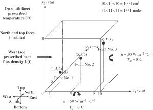
A numerical example dealing with a 3D thermal system illustrates the identification method. Though the numerical example dealt with is exactly the same as the one presented in 8, the identification method is totally different. Let us consider a cube (0.1 × 0.1 × 0.1 m³) schematically presented in figure 1. The thermal conductivity of the matter composing the cube depends linearly on the temperature according to the following law: (------120570--31) where the local temperature T is expressed in °C. The transient nonlinear energy equation, which takes the form of equation (1), is written as: (------120570--32) where T = (x, t) with x = (x₁, x₂, x₃) and ρC_p = 4.029 × 10⁶ J m⁻³ °C⁻¹. The associated boundary conditions are given by: (------120570--33-) (------120570--33-) (------120570--33-) (------120570--33-) (------120570--33-) (------120570--33-) where T_∞ = 0°C is the ambient temperature surrounding the east and bottom faces, and h = 50 W m⁻² °C⁻¹ is a convective exchange coefficient. A possible initial condition is given by the resolution of equation (32) in steady state regime, when boundary conditions given by equation (33) are applied with a given loading U(t = 0). The domain is discretized using the Finite Volumes Method 5, with 11 nodes in each direction, leading to a DM given by equation (5) of order N = 1331. In order to illustrate the method, let us consider three points inside the domain as schematically shown in figure 1. The first point is located near both the bottom face and the west face, where a given heat flux is prescribed. The second point is located at the exact centre of the cube. The third point is located near both the top face and the east face. Our goal is to build a RM describing the thermal behavior of these three points.

Figure 1. Test case configuration.

4.2. Identification results using the Adjoint Method and comparison with the Finite Difference Method

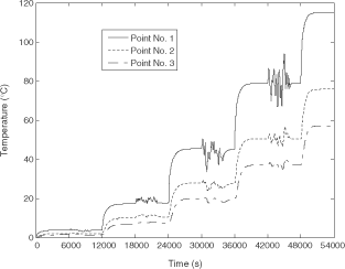
We present in figure 2 the signal U(t) used for the RM identification. The number of time steps nt equals 10800. Each step lasts for 5 s. In total, one thus gets 32403 points of temperature evolution for the three considered spatial points. Figure 3 shows the temperature response obtained with the DM of order N = 1331.

Figure 2. Heat flux density U(t) used for RM identification.

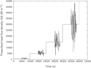
Figure 3. The DM's temperature responses at the three points when the input signal shown in figure 2 for the RM identification is applied. These temperature points along with the corresponding signal are used as data for the RM identification.

Table 1 summarizes the results of the identification of RMs of orders n = 1 to 5. For each distinct order n, the minimization of the quadratic criterion j(u) given by equation (9) is performed. The identification has been performed using two different approaches to compute the gradient of j(u): the classical FDM and the AM as developed in this article. At first, some similar observations can be made for both methods. For the first three orders from n = 1 to n = 3, the mean quadratic error characterizing the RM identification quality rapidly decreases from 1.4 to 0.02°C. For n = 4, the gain in precision is still substantial with . Increasing the order to n = 5 leaves quasi-unchanged: the identification criterion is slightly better but the improvement is not significant. That is the reason why RMs of order n = 4 will be used for the validation (section 4.3). Table 1 also allows a comparison of computing time for the RM identification when using the FDM on one hand, and the AM on the other hand for the computation of the objective function gradient. In terms of average time per iteration, it can be observed that for orders n = 1 and n = 2, the FDM is faster. For n = 3, both methods are almost as efficient, and for n = 4, the AM becomes much faster. Even though the AM is, in this special case, more efficient than the FDM only for orders greater than 2, cumulating for each method the total times needed to identify the reduced model gives the advantage to the AM. For instance the total CPU times to access the third-order RMs are equal to 1369 and 1787 s CPU for, respectively, the AM and the FDM. To access the fourth-order RM, the total CPU times are, respectively, equal to 2218 and 11050 s CPU. Let us now give pieces of information to explain these differences. Let us call m the number of parameters to be identified. One has m = n(1 + p +n(n + 1)/2). For the presented example, one has p = 1 input and m = n(2 + n(n + 1)/2). In the case of using the FDM, (m + 1) runs of the direct problem are performed at each iteration, and the direct problem itself involves a set of n coupled nonlinear differential equations of first order in time. When using the AM, two problems are performed at each iteration, whatever the value of m. The first one is the classical direct problem, and the second one is the linear adjoint problem given by equation (27). These characteristics explain the reason why the AM takes the advantage over the FDM as soon as n = 3. Actually, the AM is a little bit slower than the FDM for the first two orders. This comes from the state matrix of the adjoint problem given by equation (27), which is no longer diagonal and which also depends on time through the Jacobian . Next, in terms of absolute computing time, the AM provides an interesting gain even for n = 3. Although the time per iteration is almost identical for both approaches, the AM requires fewer iterations. Except for n = 2, this fact is verified for each value of n. This is not really surprising because the AM computes the exact objective function gradient while the FDM only leads to approximations.

Table 1. The RM identification results. Comparison between the FDM and the AM for the computation of ∇j(u).

	(K)		Number of iterations		Computing time (s CPU)		Average time per iteration (s CPU)
Reduced model order n	FDM	AM	FDM	AM	FDM	AM	FDM	AM
1	1.396	1.396	12	10	7	34	0.6	3.4
2	0.187	0.187	73	76	134	368	1.8	4.8
3	1.92 × 10^−2	1.96 × 10^−2	343	207	1646	967	4.8	4.7
4	9.29 × 10^−3	1.02 × 10^−2	277	111	9263	849	33.4	7.6
5	8.98 × 10^−3	1.01 × 10^−2	4	1	364	17	91	17

4.3. Validation of the identified RM

In order to validate the identified RM, it is necessary to test it with an input signal U(t) very different from the signal used for the model identification. Figure 4 shows a signal U(t) including steps, ramps and a sinusoid. Figure 5 shows temperature responses computed with the DM. For both approaches, the RM reproduces very efficiently the DM's behaviour. Since it is not possible to distinguish the quasi-perfectly superposed curves, we rather propose to show the discrepancies between both models on separated graphs. The discrepancies are shown in both figure 6 and 7.

Figure 4. Test heat flux density U(t) used for RM validation.

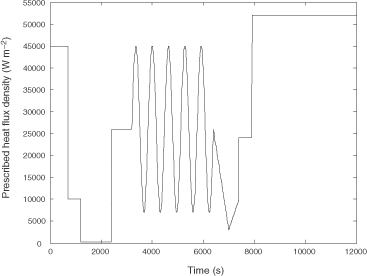
Figure 5. The DM's temperature responses at Points No. 1, 2 and 3 when the test input signal U(t) is applied.

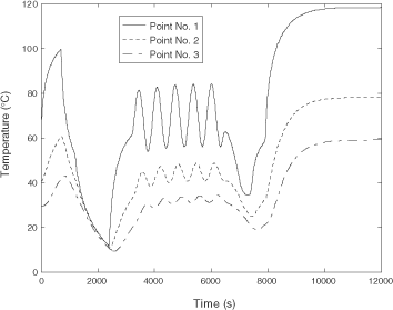
Figure 6. Discrepancies between DM's and RM's (FDM) responses when test function is applied.

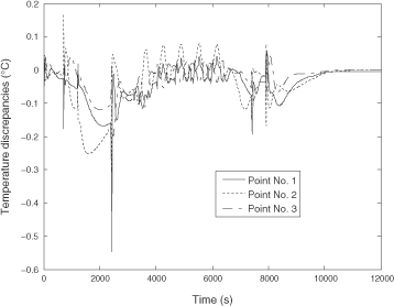
Figure 7. Discrepancies between DM's and RM's (AM) responses when test function is applied.

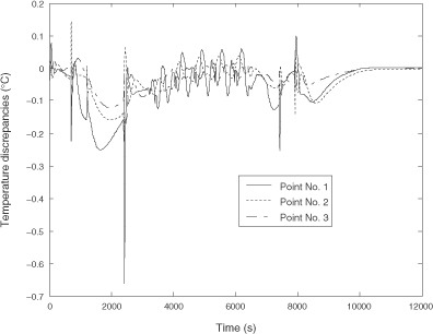
Figure 6 shows the residuals between DM's responses and those computed with the order 4 RM obtained using the FDM. Figure 7 shows the residuals between DM's responses and those computed with the order 4 RM obtained using the AM. Discrepancies are of the same order of magnitude for both the approaches. The RM built using the FDM seems slightly better for the Point number 1 while the RM built using the AM is better for Point number 2. Though the quality of the RM is almost identical for both approaches, the main difference between both approaches comes from the high time reduction when using the AM.

Next, it is pointed out that the use of the RM instead of the DM yields a drastic reduction of computation time. The direct problem resolution requires only 0.15 s CPU with a RM of order 4, instead of 163 s CPU with the original DM of order 1331. This reduction factor is greater than 1000.

Eventually, one should note the quite high level of nonlinearities in the proposed example: if the linear RM obtained by zeroing the nonlinear term ΩZ(X(t)) involved in equation (8) is used, the resulting temperature evolutions are far from those shown in figure 5, with discrepancies up to 80°C.

5. Conclusion

An approach combining the MIM for identifying nonlinear RMs and the AM for computing the gradient of the objective function to be minimized has been developed in this article. The adjoint problem is derived from the structure of the RM to be identified. This adjoint problem is linear even if the direct problem is nonlinear; it has to be solved backward in time, only once per iteration. The components of the objective function gradient are obtained through the differentiation of the lagrangian with respect to the parameters. In the end, the objective function gradient components are given through a single scalar product. The coupled method has been applied on a test case involving a 3D nonlinear transient heat conduction problem, with thermal conductivity being temperature dependent. A comparison has been made between the proposed Adjoint approach and the FDM for the objective function gradient computation. Both approaches have led to similar results in terms of Model Reduction quality. However, the AM has greatly reduced the computation time since only two problems (direct and adjoint problems) have to be solved at each iteration whatever the number of unknown parameters. The accuracy of identified RMs has also been shown, with drastic reduction of computation time when using the RMs instead of the original DM. Of course the workability of the proposed approach has been demonstrated only on a single 3D nonlinear unsteady conduction problem. Though the presented test case may be not representative enough, the authors are currently testing the adjoint method on forced convection problems where a large number of parameters are to be identified. The preliminary results are very promising. Further studies shall concern the model reduction for other fluid mechanics problems and especially on the use of the adjoint theory for the control of some fluid flows.

Additional information

Notes on contributors

M. Girault§

§Present address: From October 2004, the author has been staying at the Laboratoire d’Energétique et de Mécanique Théorique et Appliquée, UMR CNRS 7563-2, Avenue de la Forêt de Haye, BP 160, 54504 Vandoeuvre les Nancy – France.

Notes

§Present address: From October 2004, the author has been staying at the Laboratoire d’Energétique et de Mécanique Théorique et Appliquée, UMR CNRS 7563-2, Avenue de la Forêt de Haye, BP 160, 54504 Vandoeuvre les Nancy – France.

References

- Videcoq, E, and Petit, D, 2001. Model reduction for the resolution of multidimensional inverse heat conduction problems, International Journal of Heat and Mass Transfer 44 (2001), pp. 1899–1911.
- Girault, M, Petit, D, and Videcoq, E, 2003. The use of model reduction and function decomposition for identifying boundary conditions of a linear thermal system, Inverse Problems in Engineering 11 (2003), pp. 425–455.
- Bay, F, Labbé, V, Favennec, Y, and Chenot, JL, 2003. A numerical Model for Induction Heating Processes Coupling Electromagnetism and Thermomechanics, International Journal of Numerical Methods in Engineering 58 (6) (2003), pp. 839–867.
- Sophy, T, and Sadat, H, 2002. A three dimensional formulation of a meshless method for solving fluid flow and heat transfer problems, Numerical Heat Transfer, Part B: Fundamentals 41 (5) (2002), pp. 433–445.
- Patankar, SV, 1980. "Numerical heat transfer and fluid flow". In: Series in Computational Methods in Mechanics and Thermal Sciences. New York: Hemisphere; 1980.
- Favennec, Y, The comparison between the discretized continuous gradient and the discrete gradient when dealing with nonlinear parabolic problems, Numerical Heat Transfer, Part B: Fundamentals, (Accepted, to appear in 2005).
- Girault, M, and Petit, D, 2005. Identification methods in nonlinear heat conduction – Part 1: model reduction, International Journal of Heat and Mass Transfer 48 (1) (2005), pp. 105–118.
- Girault, M, and Petit, D, 2005. Identification methods in nonlinear heat conduction – Part 2: inverse problem using a reduced problem, International Journal of Heat and Mass Transfer 48 (1) (2005), pp. 119–133.
- Marshall, SA, 1966. An approximate method for reducing the order of a linear system, Control (1966), pp. 642–643.
- Aoki, M, 1968. Control of large-scale dynamic systems by aggregation, IEEE Transactions on Automatic Control 13 (3) (1968), pp. 246–253.
- Litz, L, 1981. Order reduction of linear state space models via optimal approximation of the nondominant modes, North-Holland Publishing Company Large Scale System 2 (1981), pp. 171–184.
- Newman, AJ, Model reduction via the Karhunen–Loève expansion, Part I: an exposition. Presented at Technical Research Report of the Institute for Systems Research. 1996, (http://techreports.isr.umd.edu/TechReports/ISR/1996/TR_96-32/TR_96-32.phtml).
- Neveu, A, El-Khoury, K, and Flament, B, 1999. Simulation de la conduction non linéaire en régime variable: décomposition sur les modes de branche. Simulation of nonlinear non-steady-state conduction: expansion on the branch modes, International Journal of Thermal Sciences 38 (4) (1999), pp. 289–304.
- Girault, M, and Petit, D, 2004. Resolution of linear inverse forced convection problems using model reduction by the Modal Identification Method: application to turbulent flow in parallel-plate duct, International Journal of Heat and Mass Transfer 47 (17–18) (2004), pp. 3909–3925.
- Gill, PE, Murray, W, and Wright, MH, 1992. Practical Optimization. London, UK: Academic; 1992.
- Michaleris, P, Tortorelli, DA, and Vidal, C, 1994. Tangent operator and design sensitivity formulations for transient non-linear coupled problems with applications to elastoplasticity, International Journal of Numerical Methods in Engineering 37 (1994), pp. 2471–2499.
- Tortorelli, DA, and Michaleris, P, 1994. Design sensitivity analysis: overview and review, Inverse Problems in Engineering 1 (1994), pp. 71–105.
- Woodbury, KA, 2002. Inverse Analysis Handbook. Boca Raton, FL: CRC Press; 2002.
- Favennec, Y, Labbé, V, and Bay, F, 2003. Induction heating processes optimization – a general optimal control approach, Journal of Computational Physics 187 (2003), pp. 68–94.
- Favennec, Y, Labbé, V, and Bay, F, 2004. The ultraweak time coupling in nonlinear multiphysics modelling and related optimization problems, International Journal for Numerical Methods in Engineering 60 (2004), pp. 803–831.
- Céa, J, 1971. Optimisation, théorie et algorithmes. Paris: Dunod; 1971.
- Larrouturou, B, and Lions, PL, 1994. Méthodes mathématiques pour les sciences de l’ingénieur: optimisation et analyse numérique. Cours de l’Ecole Polytechnique; 1994.
- Jarny, Y, Ozisik, MN, and Bardon, JP, 1991. A general optimization method using adjoint equation for solving multidimensional inverse heat conduction, International Journal of Heat and Mass Transfer 34 (11) (1991), pp. 2911–2919.
- Minoux, M, 1986. Mathematical Programming – Theory and Algorithms. Chichester: John Wiley and Sons; 1986.