Estimation of a source term in a two-dimensional heat transfer problem: application to an electron beam welding

Abstract

This article is concerned with the estimation of a heat source applied in the electron beam welding process by using the micrographic information (hardness, optical micrograph, etc.) and temperature measurements in solid phase. The aim is to identify the energy distribution that is applied in the liquid and vapor zones. This identification is realized at each time in a transversal plane perpendicular to the welding axis. For this work, the goal is to analyze the feasibility of the estimation. So we do not use noise with the theoretical measurements. At last, the iterative regularization method will be used for this two-dimensional metallurgical inverse heat transfer problem.

Keywords:

• Electron beam welding
• Heat Affected Zone (HAZ)
• Thermocouple

1. Introduction

Welding is an assembling operation that affects both mechanical and structural properties and which is very sensitive to control parameters of technological processes. The first stage of this study is to choose these parameters which lead to an acceptable welding quality. The main difficulty of the theoretical analysis is that the exact distribution of the thermal energy absorbed and generated in the liquid and vapor zones is not easy to predict and cannot be measured directly. When studying the welding, the theoretical analysis use complementary experimental information: the temperature measurements near the liquid zone and the microstructural properties (hardness, optical micrograph, etc.).

The objective of this work is the estimation of the energy distribution in the welding zone. The temperature difference between the welding and solid zones is big enough, but there is a strong damping effect in the solid zone. That is why it is difficult to estimate correctly the energy distribution from the temperature measurements taken at points that are too far from the welding zone.

Many works deal with the estimation of boundary conditions or the determination of distributed heat flux on the boundary of the body [1–3]. Few of these works consider experimental situations involving unknown heat sources. Silva Neto and Ozisik [4] used the conjugate gradient algorithm to estimate the time-varying strength of a line source placed in a rectangular region with insulated boundaries, but the location of the source was specified. Le Niliot [5] studied linear inverse problems with two point heat sources, and experimental results were presented in [6].

In many studies, the inverse fusion and solidification problem have been analyzed which use a simplified approach based on only a conduction model in the liquid and vapor zones. Under these assumptions, 1D or 2D Stefan problems taking into account only the conduction effects in all the phases during the process were considered. The objective was to estimate an energy distribution [3], or a motion of the solid–liquid interface [7–10]. Another approach was to take into account the convection effects described by the Navier–Stokes equations in the liquid and vapor zones [11]. At last, mixed approaches were employed, in which an apparent source term is determined in the liquid and vapor zones representing the different phenomena [12].

In this article, we use the first hypothesis for the electron beam (EEB) welding process. We consider only the conduction effects for all phases (solid, liquid and vapor). The iterative regularization method [2] is used to estimate the dissipation energy in the liquid and vapor zones. First, we present the EB welding technique and the used steel sample. Second, we describe the direct problem including the simulation of phase transformations and the source term (EB). Third, the estimation procedure is described. Finally, the estimation results are discussed.

2. The electron beam welding

2.1. Principle

The EB welding is an assembling process in vacuum using a high density energy beam. This technique permits the welding of the high thicknesses (up to 16 cm) with a low width and a narrow Heat Affected Zone (HAZ). At the beginning of the welding process, the high power density of the electron beam leads to an evaporation of the material and then to a keyhole (figure 1). It is this keyhole and its displacement that generate the welded joint. The high penetration capacity of the beam with a narrow fusion zone characterizes the EB welding in comparison with other weld methods. For these other methods, the penetration is limited by the heat conduction [13].

Figure 1. Welding process.

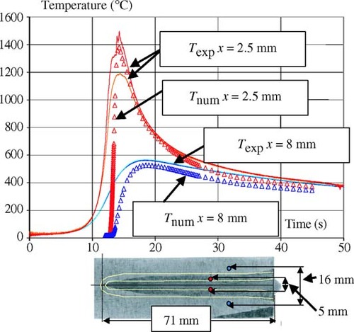
For this study, weld joints are used which are realised in the “Direction des Constructions Navales” (DCN) in Indret (44-France) (power of this electron beam: 100 kW). The welds are made of 18MnNiMo 5 steel samples (ASTM A508 Cl.3) or with aluminum samples. In this article, a partial penetration welded joint is analyzed. Figure 2 shows the micrography of this sample which is used to determine precisely the locations of the measurement points by using a scan of this welding joint. The welding parameters are: voltage U = 60 kV, current I = 0.29 A, velocity v = 2.5 mm s⁻¹, focus current If = 2.46 A. The work of Carin et al. [14] presents the experimental parts of this study.

Figure 2. Weld joint (dimensions in mm).

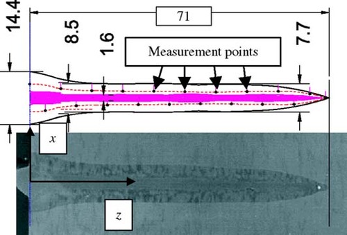
The high temperature level in the fusion and vapor zones prevents the installation of the thermocouples in these zones. The used thermocouples (d = 80 µm; K type, C type or S type) are thus located in the HAZ (750°C<T<1450°C). Figure 2 and table 1 show the positions of measurement points.

With the experimental temperatures obtained from the thermocouples and corresponding diagrams (CCT or TTT) we will validate the simulation of the metallurgical transformations by comparing the experimental and simulated thermal and metallurgical parameters. Furthermore, temperatures computed at the thermocouple locations by solving the direct problem will be used to estimate the source term in the fusion and vapor zones.

Table 1. Thermocouple locations.

Thermocouple i	1	2	3	4	5	6	7	8	9	10	11	12	13	14	15	16	17
xi (mm)	2.38	2.38	2.38	1.95	1.95	1.95	1.58	1.58	1.58	1.25	1.25	0.98	0.75	0.58	0.45	0.23	0
zi (mm)	0	4	8	12	16	20	24	28	32	36	40	44	48	52	56	60	64

2.2. Numerical simulation of the electron beam welding

Several works are concerned with the numerical simulation of the EB welding in the laboratory LET2E [15]. In these works, the SYSWELD code [16] was used. In this study, we use a new code analogous to SYSWELD which is incorporated in the developed estimation code. The finite difference method based on an implicit scheme is used to solve the direct and inverse problems. The equations are the heat conduction equation (1)(1) and the metallurgical kinetic equations (2)(2) of the type Leblond and Devaux [17], and Koistinen and Marburger [18]. The studied domain is one-half of the transversal plane taken perpendicular to the welding axis (figure 3), (1) (phase no. 1 = ferrite–perlite, phase no. 2 = bainite, phase no. 3 = martensite and phase no. 4 = austenite) (2) The boundary and initial conditions are the following: at the lower, upper and lateral surfaces, only the radiative conditions are fixed because the welding process is carried out in vacuum. 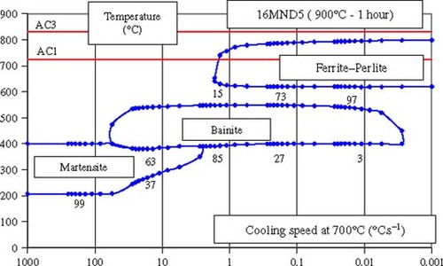For example at the lower surface, the boundary condition is: (3) On the axis: (4) Initial conditions: (5) In the heat conduction equation (1)(1) , the source terms (∂ Pα /∂ t)Lα γ (T) and ∂ (ρ H)/∂ t allow to take into account the phase change enthalpy according to the temperature of the sample (metallurgical transformations for the first term, fusion and evaporation for the second). The transformation energy is calculated according to the phase enthalpy: Lα γ (T) = ργ Hγ − ρα Hα and by considering two metallurgical phases only: γ (austenite) and α (ferrite, perlite, bainite or martensite). The enthalpies of the phases α and γ are computed with the use of polynomial functions between 100 and 1450°C. The parameters of the metallurgical kinetic equations are calculated by simulating the CCT diagram (example: figure 4).

Figure 3. Definition of the study plane.

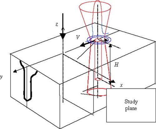
Figure 4. CCT diagram.

For each time and space node, the cooling speed and the temperature value are used. With this information, the percentage Pi of the metallurgical transformation is computed. Moreover, the thermophysical characteristics ρ(T ), C(T ) and λ(T ) are calculated at all time steps by a law of mixtures according to the temperature (example: λ(T)  = Pγ × λγ (T ) + Pα × λα (T)  = Σi Pi λ (T)).

For the phase γ and for T<1450°C: (6) For the phase α and for T<750°C: (7) The other thermal transformations are computed between 1450 and 1550°C for the fusion and between 2600 and 2800°C for the evaporation. These enthalpies are given in Costantini's work [13]: ΔHfus = 391970 J kg⁻¹ and ΔHvap = 6332879 J kg⁻¹. At last, the thermophysical characteristics of the liquid and vapor phases are computed at 1450°C.

The initial data of the model are:

a.	The mesh;
b.	The thermophysical characteristics ρ(T ), C(T ), λ(T ), and Lαγ for the different phases according to the temperature;
c.	The initial and final temperatures of thermal transformations for all phases (CCT diagram);
d.	The initial temperature T0 = 20°C in whole domain;
e.	The ambient temperature Tinf;
f.	The emissivity of the considered material is supposed to be constant and equal to 0.8.

The set of equations is solved with the use of a fine discretization of the domain near the EB zone (176 nodes in the vertical direction; 52 nodes in the transverse direction). The finite difference grid is uniform in the vertical direction, Δz = 0.5 mm, and not uniform in the transverse direction, 0.05 mm<Δx<2 mm. The direct problem and the corresponding code have been verified in previous papers [15].

Figure 5 shows the comparison between the experimental data and numerical results for a Gaussian source [14]. Globally, we find a good level for the maximal temperatures. Some problems stay because, in this 2D transverse model, we do not have the diffusion effect forward the beam. For this reason, it seems to be important to estimate an apparent source term for modeling the diffusion effect in the steel.

Figure 5. Comparison between the experimental and numerical temperatures.

3. Estimation algorithm

The objective of this research is to determine a source term S(x, z, t). The determination is conducted from the temperature values measured in the HAZ at a distance between 3 and 10 mm from the welding axis. The time step used in the estimation is Δt = 0.001 s and the discretization on the welding axis is Δz = 0.5 mm and Δx = 0.5 mm.

3.1. Minimization procedure

The use of the iterative regularization method leads to the variational formulation of the inverse problem of estimating the source term and the residual functional minimization by utilizing the unconstrained conjugate gradient method. The residual functional is defined as: (8) where T(xj, zj, t; S) and Yj (t) are the computed and measured temperature histories respectively at N various measurement points of the material. The inverse algorithm consists in minimizing this residual functional under constraints on the temperature given by the direct problem (equations (1)(1) to (7)(7) ).

The function S(z, x, t) is considered as an element of the Hilbert space L². The source term is computed as a grid function. In the iterative method, the desired function approximations are built at each iteration as follows: (9) where n is the iteration index, n* is the index of the last iteration, γ ⁿ is the descent parameter, Dⁿ is the descent direction given by: (10) where: (11) ⟨,⟩ is the scalar product in Hilbert space L², S ⁰ is an initial approximation of the function to be estimated given a priori.

In the absence of noise, the iteration procedure is carried on until the following stopping criterion is verified: (12) The residual functional gradient ∇ Jⁿ is calculated at each computational grid node (x, z, t) by the following analytical relationship: (13) where Ψ(x, z, t) is the solution of the following adjoint problem derived by using the approach given in [2]: (14) (15) (16) (17) (18) (19) The descent parameter of γ ⁿ is computed as follows: (20) where θ(x, z, t) is the solution of the following direct problem in variations: (21) (22) (23) (24) (25) (26) where δS(x, z, t) = Dⁿ(x, z, t).

The variation problem is obtained with a variation δS of the source term S(x, z, t). In that case, the temperature T(x, z, t) is perturbed by a variation θ(x, z, t). Writing equations (1)(1) to (5)(5) for the perturbed solution and subtracting the same equations for the solution T, we obtain the variation problem. For example: (27)

3.2. Regularization

The inverse problems are ill-posed and numerical solutions depend on the fluctuations occurring at the measurements. Small fluctuations at the measurements can generate big errors in the inverse problem solution. So regularization is needed to stabilize the solution. According to the iterative regularization method, the regularizing discrepancy criterion is used for the stabilization: (28) where (29) σ²(xj, zj, t) is the standard deviation of the temperature measurement errors. The index n* is the index of the last iteration. For this index, the equation (28)(28) is validated and n* is defined as the regularization parameter in the method.

3.3. Computational scheme

The three systems (direct, adjoint and variation problems) are solved numerically using a finite difference method and an implicit scheme. The estimation procedure consists of the following steps:

1.	Define the initial values of S 0(x, z, t)
2.	Solve the direct system: equations (1)(1) to (7)(7)
3.	Calculate the residual functional criterion J(S): equation (8)(8)
4.	Verify the stopping criterion: equation (12)(12) or (28)(28) . If the stopping criterion is verified: go to step (12) otherwise go to step (5)
5.	Solve the adjoint problem: equations (14)(14) to (19)(19)
6.	Calculate the residual functional gradient: equation (13)(13)
7.	Calculate the descent direction: equations (10)(10) and (11)(11)
8.	Solve the direct problem in variations: equations (21)(21) to (26)(26)
9.	Calculate the descent parameter γn: equation (20)(20)
10.	Improve the desired function S n+1(x, z, t): equation (9)(9)
11.	Go to step (2)
12.	Stop

4. Numerical simulation

To verify the numerical algorithm, two test cases with fixed exact forms of the source term given a priori are analyzed.

The first form is defined by: (30) The source term is a source imposed in x = 0 which varies linearly with z (figure 6). This source gives a small fused zone (Δx = 0.75 mm; Δz = 1.5 cm) and the maximum temperature at the point x = 0, z = 0 is equal to 1650°C. The heat distribution crosses the analyzed transversal plane in 25 s. The computational time step is equal to 0.05 s. For the estimation, we use only the exact measurements computed in the HAZ in 25 s (figure 7). In fact, we have chosen these parameters for the verification of the computational algorithm. One parameter that characterizes the difficulty of the inverse problem solution is the number ΔF0 = aΔt/Δx². This number is calculated with average values: a = 5 × 10⁻⁶ m² s⁻¹ (thermal diffusivity), Δx = 0.75 mm (minimum distance between the measurement points and the axis), Δt = 0.05 s (time step) and we obtain ΔF0 = 0.44. Generally, we have no problem for the source estimation when the Fourier number is greater than 0.1.

Figure 6. First form.

Figure 7. Computed temperatures.

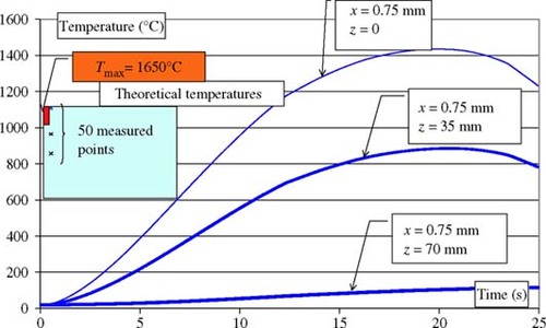
Figure 7 shows the temperature histories for three measured points taken on a vertical line near the fused zone. The difference between the maximum temperatures in the axis x = 0, z = 0 and in the first measurement point x = 0.75 mm, z = 0 is equal to 200°C. So, the damping effect is low in this case. The analysis of the estimation results (figure 8) shows that the algorithm is correct. The maximum residual between the estimated and exact energy distribution is less than 1% (figure 9).

Figure 8. Estimated source.

Figure 9. Residual between the exact and estimated sources.

The second form is a Gaussian source, which corresponds to several studies carried out in the laboratory LET2E [15]: (31) where the parameters are: efficiency coefficient η = 0.9, voltage U = 60 kV, current Ib = 0.29 A, velocity v = 2.5 mm s⁻¹, penetration h = 7.1 cm, beam diameter Φ = 0.6 mm.

The Gaussian source is divided in two parts. The first one Sv (most energetic part) (figures 10 and 11) is applied in the domain where it goes inside the material (creation of the keyhole). The second one Ss (a ring shape – figure 10) is only a surface heat source corresponding to the “non active” part of the beam. In this article, we deal only with the estimation of the most energetic part. With these distributions, we can obtain simulated fused and HAZs close enough to those shown in figure 2 [14].

Figure 10. Source definition.

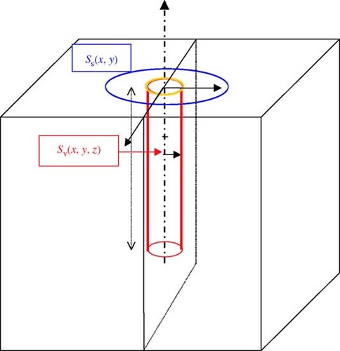
Figure 11. Exact Gaussian source in z = 0.

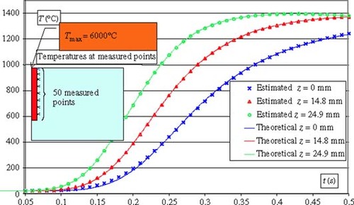
Here again, we use, for the estimation, only the exact measurements computed in the HAZ in 0.5 s. This time corresponds to the crossing of the analyzed plane by the beam (0<t<0.35 s) and the beginning of the cooling. Figure 12 shows three computed temperature histories taken in the HAZ. The maximum temperature is around 1400°C. On the welding axis the maximum calculated temperature is around 6000°C, which demonstrates the high damping in the material. In this case, the Fourier number is calculated with average values: a = 5 × 10⁻⁶ m² s⁻¹, Δx = 1.5 mm, Δt = 0.001 s and it is equal to ΔF0 = 0.002.

Figure 12. Comparison of the temperatures.

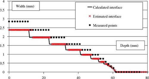
The analysis of the estimation results (figures 12–15) permits to underscore the following points. If we compare the exact and estimated temperatures, it can be seen that the results are good enough. But after 200 iterations (figure 13), we do not correctly find the Gaussian shape of the source term in transversal direction (figure 14). Globally, we find the average values of the source. On the other hand, the Gaussian form as a function of time is correct. An analysis of this mean heat distribution depending on the depth shows that the estimated form follows well the exact function f (z) = 1 − (z/h). Another comparison point is the boundary of the fusion zone. Figure 15 shows these exact and estimated boundaries. In the scale of the computational finite difference grid, the shape is followed well. Finally, one can see that it is more difficult to obtain the convergence to the exact source term for the beginning of the welding process. This difficulty comes from the fact that there is no conduction effect forward the beam (only a transversal plane is analyzed). So, the temperature variation is very abrupt when the beam arrives at the study plane. In reality, the thermocouples give information on the beam due to the conduction effects and it is easier to estimate the source term at the beginning of the welding process.

Figure 13. The residual functional evolution.

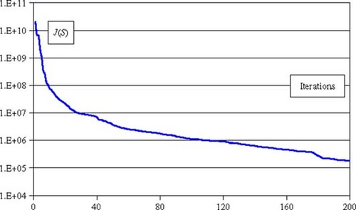
Figure 14. Estimated source in z = 0.

Figure 15. Evolution of the fused zone.

5. Perspectives

A quasi-stationary simulation in a longitudinal plane will be realized. A similar approach is used in [14]. This study permits consideration of the conduction effects in the beam front. To do that, the inverse algorithm was modified in the direct, the variation and the adjoint problems. This work will be carried on with a 2D or 3D quasi-stationary simulation. The objective of these studies is to estimate the heat flux in the fusion zone, by using the temperature measurements in the HAZ. To ameliorate the convergence of the algorithm, we are going to take into account the interface locations between the fusion and the HAZs. Then, the simulated noised temperature evolutions will be used to verify the method. At present, we develop an experimental setup to obtain experimental data. The final objective is to estimate a source term in the fusion zone and the shape of this zone.

6. Conclusion

The goal of this work was to establish a methodology for the estimation of the energy distribution in an EB welding operation. Two test cases with exact forms of the source term given a priori were chosen to verify the developed estimation method. The first exact form was a line source in x = 0 and a sinusoidal form in function of time. This source crosses the transversal plane in 25 s. This configuration gives a ΔF0 number equal to 0.44 and shows the robustness of the computational algorithm. The second test case, a Gaussian distribution, was chosen to simulate numerically the beam. The estimation results show that it is difficult enough to obtain a true distribution in the transverse direction (x-direction) with a number ΔF0 = 0.002. On the other hand, the estimated distribution in other directions (time and depth) is good enough. This work will be continued with the use of the experimental microstructural information (the boundary of the fusion zone, the boundary of the HAZ, hardness, etc.).

Nomenclature

Table

a	thermal diffusivity (m^2 s^−1)
Ci	specific heat of the phase i (J kg^−1 K^−1)
D^n	vector of descent direction
dT/dt	variation of the temperature with time (K s^−1)
Δ F0 = a Δ t/Δ x^2	delta Fourier number
h	penetration (m)
Hγ, Hα	enthalpies of the phases γ and α (J m^−3)
ΔHfus, ΔHvap	enthalpies of the phase change (J kg^−1)
I, If	current and focus current (A)
J(S)	residual functional
∇ J^n	the gradient of the residual functional
Lij, Lγ α	heat transformation of phase i to j (J m^−3)
n, n*	iteration number, last iteration
Pi, P, Peq	proportion of metallurgic phase (per volume fraction)
Pij	proportion of the transformed phase i to j
x	spatial coordinates (m)
S^n^+1, S(x, z, t)	source term
Tinf	external temperature (°C).
T, Ti	temperature in the sample (°C)
T0	initial temperature in the sample (°C)
U	voltage (V)
v	velocity (m s^−1)
Y, Yi, Ye	experimental temperatures (°C)
z	spatial coordinates (m).
γ^n	descent parameter
δ^2	convergence criterion
ε(T)	emissivity of the sample
ε1	arrest criterion
η	efficiency coefficient
λi	conductivity of the phase i (W m^−1 K^−1)
ρi	density of the phase i (kg m^−3)
σ^2	standard deviation of the temperature measurement errors
ω	a random number
θ(z, r, t)	temperature variation
Φ	beam diameter (m)
Ψ(z, r, t)	adjoint variable

Acknowledgements

The authors acknowledge the CESMAN – DCN Indret for the weld joints.