Abstract
A modal method combined with system condensation is presented for the assessment of selection optimality and solution accuracy in inverse problems of structural optimization and damage detection. Finite element procedures are applied to seek the structural modifications for the characteristic changes assigned from design goals or dynamic measurements. The solution convergence is related to the selection of degrees of freedom and the method of system transformation. The application of the dynamic stiffness matrix yields a frequency-dependent transformation matrix, which can be expanded into an infinite series to obtain lower-order approximations. The modal matrix may be used to project the measured data onto the mode shapes, in which case much emphasis is laid on the linear independence of the selected degrees of freedom and the condition number of the transformation matrix. The baseline structure is used to obtain an initial perturbation, which can be improved through repeated updates of the transformation. The proposed methods give excellent solutions for frequency optimization. In damage detection, however, moderate deviations from the correct structural changes are attributable to system reduction. The dynamic stiffness matrix seems recommendable over the modal matrix projection for the system transformation.
1. Introduction
Finite element theories coupled with advanced computer technologies and efficient numerical algorithms have made it feasible to explore the structural problems of large and complex systems in more depth. Continuous material and geometric properties are discretized to yield a set of system equations, which is solved to get the desired static and dynamic responses.
In general, dynamic analysis of large structures takes much computing time and resources. For linear eigenproblems, various condensation methods Citation1–7 are applied to obtain the lowest modes with accuracy acceptable in an engineering sense. The mode shape is approximated by a small set of primary (master) degrees of freedom whereas secondary (slave) ones are condensed out. The original system is reduced into a subspace of the primary set. The condensation procedure is straightforward and gives a unique solution in analysis problems.
Over the past few decades, the finite element method has been extended to the inverse problem of structural optimization Citation8–10, system identification Citation11–13, and damage detection Citation14–16. In conventional modal methods, the perturbations in modal characteristics (natural frequencies and mode shapes) are related to the modifications of structural properties (stiffness and mass). In spite of numerous difficulties in problem formulations and engineering tests, the abundance of modal data has been a strong driving force behind the research work on the methods. The theoretical equations are complicated and the inverse solution may not be unique Citation17.
As is well known, the accuracy of eigenvalue is of the second order whereas the eigenvector shows an error of the first order Citation18. Typical measurements show approximately 0.1 and 10% errors for the natural frequency and mode shape Citation19. Hence, the eigenvalue related to the modal energy is preferred over the mode shape in inverse formulations and excellent results can be obtained in structural optimization for frequency changes.
A minor difficulty arises from the fact that the energy equation is, mathematically, only a necessary condition for the system equilibrium. In a physical sense, the total energy of an eigenmode is the sum of energies of all elements or degrees of freedom. The perturbations of local elements are added together to yield the global eigenvalue change and hence, natural frequencies are less sensitive to each element change.
Care should be taken with the degrees of freedom in mode shapes. In structural optimization, a set of primary degrees of freedom can be specified as desired for design goals. Dynamic sensors are placed on the measurable degrees of freedom of the accessible nodes in engineering tests for system identification and damage detection. Although the computational efficiency is enhanced through system condensation, the consequent solution error is, to some extent, unavoidable. Hence, a direct approach Citation20 was applied to extract the equilibrium equations of the primary degrees of freedom for converged solutions in inverse problems.
The application of dynamic stiffness matrix yields a frequency-dependent transformation between the primary and secondary sets. For simplicity, however, lower-order approximations are obtained in an infinite series expansion. The rate of convergence depends on the smallest eigenvalue in the subspace of the secondary structural matrices. The ratios mii/kii or the energies associated with degrees of freedom can be used as a guideline Citation21–24 for the selection of a primary set or the elimination of a secondary one.
In the case where the modal matrix is employed to project the given primary data onto the mode shape, the transformation usually becomes overdetermined because more sensors than modes are placed to secure the accuracy of the measured data. Hence, a pseudo-inverse is introduced for the least squares approximation and the linear independence of the primary degrees of freedom is of great importance. The left singular vectors obtained through singular value decomposition of the modal matrix can be used to select appropriate primary sets.
The condition number of the transformation matrix dictates the numerical stability of an inverse solution. Depending on scaling and dimension of matrix, the determinant is not a good measure of ill-conditioning. Since the condition number is usually defined as the ratio of the largest and smallest eigenvalues Citation25, Citation26, Gerschgorin's theorem Citation27 can be employed to achieve a close distribution of eigenvalues and minimum condition number.
The selection of a small primary set is more competitive than the elimination of a large secondary one in terms of the computational efficiency. For the solution accuracy, however, sequential elimination seems to be superior to simultaneous selection. Sequential selection for maximum linear independence and minimum condition number shows good convergence Citation28.
The objective function of least structural changes in mathematical programming tends to scatter the element modifications over the entire structure, which may be desirable in structural optimization but rather misleading in the search for unique element modifications. The minimization of structural variables has an effect of preventing excessive variations in iterations with updated inverse systems.
Numerical examples show that the selected primary sets give excellent inverse solutions for frequency optimization, regardless of the method of system transformation. In damage detection, however, the dynamic stiffness matrix seems recommendable over the modal matrix projection. On the other hand, no significant differences can be observed between the selection criteria; maximization of the smallest eigenvalue in the secondary subspace, maximum independence of the primary modes, and minimum condition number of the transformation matrix.
Further research works are required to secure the solution accuracy in inverse problems for large structures. Also, the numerical stability of the inverse solution, in particular, in system identification and damage detection is of great importance because small errors in measured data may lead the inverse system to considerable deviations from the correct perturbed structure.
2. System condensations
2.1. Analysis problems
In linear dynamic analysis, the equilibrium equation of undamped free vibration is written as a general eigenproblem:
(------147296--1)
where k and m are the stiffness and mass matrices. An eigenpair is given as λ and ϕ.
In system condensations, the mode shape is expressed in terms of an approximation of the primary (master) degrees of freedom and the secondary (slave) ones are condensed out of the equation formulation.
(------147296--2)
where E and T are the transformation matrices for the primary and secondary sets, ϕp and ϕs. The system transformation is conducted through the use of Tp.
Substituting equation (2) into equation (1) gives a residual error in the system equilibrium.
(------147296--3)
If the equilibrium error weighted by (Tp)T vanishes, one obtains a reduced eigenproblem.
(------147296--4)
The reduced structural matrices are written as
(------147296--5)
The subspace eigenproblem of equation (4) is solved to obtain λapp and (ϕp)app. The analysis procedure is straightforward and the modal solution is unique. It should be noted that the consequent reduction error associated with the weighting would be, to some extent, inevitable.
Ritz method can be an alternative, in which an approximate mode shape is expressed as a linear combination of assumed vectors in ZL.
(------147296--6)
The vector qL contains the generalized coordinates.
Minimization of the Rayleigh quotient associated with ϕapp yields a subspace eigenproblem.
(------147296--7)
Eigensolutions give L subspace eigenvectors QL for the approximation.
(------147296--8)
In the subspace iteration method, the inverse iteration pushes Φapp further towards the exact eigenvectors and the assumed vectors are updated to get (ZL)new.
(------147296--9)
2.2. Inverse problems
Modifications of the baseline structure yield a perturbed system:
(------147296--10)
In modal methods, an inverse system of perturbed structural matrices k′ and m′ is sought for the specified modal characteristics λ′ and ϕ′. Mathematically, the force equation (10) constitutes the necessary and sufficient conditions for the system equilibrium. Physically, an inverse solution will provide a structural system with the assigned modal responses.
Premultiplication of equation (10) by (ϕ′)T gives a single equation,
(------147296--11)
which represents the equilibrium between the strain and kinetic energies of an eigenmode.
Equation(11) is only a necessary condition for the system equilibrium and hence, the structural matrices k′ and m′ do not guarantee the given eigenpair λ′ and ϕ′. Since the modal energy is the sum of energies of all elements or degrees of freedom, the effects of element modifications are mixed up together to yield the energy and eigenvalue changes. Therefore, the energy equation does not provide clear and distinct information about each element change and may be used as a supplement to accelerate the solution convergence Citation20.
In the case of a given primary set , the perturbed mode shape can be written as
(------147296--12)
where
is the system transformation matrix.
For a given eigenvalue , the system reduction gives a subspace eigenproblem:
(------147296--13)
where the reduced structural matrices are written as
(------147296--14)
The reduced eigenproblem of equation (13) is solved for the structural variables in k′ and m′. When the inverse problem is underdetermined as in structural optimization, mathematical programming techniques are often employed to get an optimal solution for an objective function of minimum weight or least structural changes from the baseline system.
Usually in inverse problems, the baseline mode shapes are available and the perturbed mode shape can be expressed as
(------147296--15)
where ΦL is the modal matrix that consists of L lowest mode shapes and qL represents a set of unknown generalized coordinates.
The dynamic reduction yields a subspace eigenproblem, in which the generalized coordinates represent the eigenvector.
(------147296--16)
In a typical problem of frequency optimization Citation29, the inverse systems of k′ and m′ always showed lower (more negative) eigenvalues although the reduced equation (16) was satisfied exactly. The solution error was caused by the truncation of higher modes in the expansion rather than a loss of accuracy in the equation solver.
3. Transformation matrices
3.1. Application of dynamic stiffness matrix
The equilibrium equation (1) can be rewritten as
(------147296--17)
where D is called the dynamic stiffness matrix.
Equation (17) is expressed in partitioned form as
(------147296--18)
The second equation gives the relation between the primary and secondary sets.
(------147296--19)
where the transformation matrix is written as
(------147296--20)
An infinite series expansion of matrix inversion shows
(------147296--21)
which converges if all the eigenvalues of A are smaller than unity.
Then, the matrix inverse in equation (20) can be expressed as an infinite series:
(------147296--22)
Substituting equation (22) into equation (20) gives
(------147296--23)
where
(------147296--24)
Note that the transformation matrix T is frequency-dependent and differs from mode to mode.
In Guyan's static condensation, the masses of the secondary set are neglected to obtain
(------147296--25)
Then, the reduced equation (4) becomes
(------147296--26)
where
(------147296--27)
Note that the matrix products containing (kss)−1can be a significant computational burden. In addition, the reduced matrices may lose the bandedness of the original structural matrices.
Equation (26) can be rewritten as
(------147296--28)
Then, the eigenvalue in equation (23) is eliminated to get an approximation
(------147296--29)
The transformation is constant and hence, in principle, applicable to all modes. In practice, however, the formulation of CG is valid only in the lowest modes. The procedure of Improved Reduction System (IRS) takes terms up to first order.
In analysis problems, an approximation of the primary set is substituted directly into the mode shape. Hence, the system transformation is written as
(------147296--30)
In inverse problems, the transformation matrix is written as
(------147296--31)
The perturbed eigenvalues are usually given from the design goals or dynamic tests. Hence, the matrix can be approximated as
(------147296--32)
In the same way, equation (32) can be expressed in an infinite series as
(------147296--33)
where
(------147296--34)
At the initial stage, the baseline system is employed to calculate the transformation matrices.
The system transformation is written as
(------147296--35)
3.2. Projection of modal matrix
Equation (15) can be rewritten in partitioned form as
(------147296--36)
The first equation gives an approximation for the given primary set .
(------147296--37)
In practice, more sensors (primary degrees of freedom) than modes are placed for better accuracy in dynamic measurements or p > L. Then, equation (37) becomes overdetermined and the least squares solution gives
(------147296--38)
The pseudo-inverse matrix is written as
(------147296--39)
where the symmetric Fisher information matrix is defined as
(------147296--40)
Then, the transformation matrices in equation (12) are obtained as
(------147296--41)
In particular, E′ is called the Effective Independence Distribution (EID) matrix. Multiplying the EID matrix by ΦpL gives
(------147296--42)
The symmetric matrix E′ has L repeated eigenvalues of unity. The primary modes in ΦpL are the corresponding eigenvectors, which must be linearly independent.
4. Convergence and selection optimality
4.1. Secondary structural subspace
It is well known that the matrix inversion in equation (22) is valid for lower modes in which λ is smaller than the lowest eigenvalue λs of the secondary structural submatrices.
(------147296--43)
The rate of convergence depends on the ratio λ/λs and hence the primary set is selected so that λs may be maximized. In sequential elimination, the secondary degrees of freedom with the smallest ratio of mii/kii are condensed out, one by one, until the system dimension decreases to the desired number of primary degrees of freedom.
The procedure of simultaneous selection is simple but suffers from a drawback in that excessive weighting is put on the elements with larger mesh and mass, which seems quite natural but becomes defective in some typical cases Citation24. The basic principle should be based on a uniform distribution of the degrees of freedom over the entire structural system.
The selection of small primary set has an advantage of computational efficiency over the elimination of large secondary one. In terms of solution accuracy, however, the sequential elimination of secondary degrees of freedom is believed to be superior to the simultaneous selection of primary ones. In large systems, the computing time for repeated condensations can be prohibitive.
Not only the ratios of diagonal terms of structural matrices but also the energies associated with degrees of freedom can provide a good guideline for the selection or elimination of degrees of freedom. For analysis problems in which the mode shapes are not known, the procedure of inverse iteration can be used to obtain the Ritz vectors Citation30. On the other hand, the baseline mode shapes are available in inverse problems for the calculation of relevant modal energies.
4.2. Linear independence
Since the Fisher information matrix S shares the same rank as ΦpL, the linear independence of the primary modes in ΦpL is very important to get nonsingular S and consequently to calculate the transformation matrices E′ and T′. The column rank of ΦL is L and so is the row rank. Hence, a proper selection of primary rows of ΦL will yield ΦpL of the full rank L.
The singular value decomposition of ΦL gives
(------147296--44)
The matrices U and V contain the left and right singular vectors, u1, … , un and v1, … , vL, which form orthonormal bases for the column and row spaces of ΦL. The diagonal matrix Σ consists of the non-zero singular values σ1, … , σL.
If the left singular vectors associated with zero singular values are omitted, a simple expression (thin form) can be obtained in terms of u1, … , uL and v1, … ,vL:
(------147296--45)
and in transposed form
(------147296--46)
Equation (46) states that each component of ui indicates the contribution of a basis vector vi to each row of ΦL. In other words, the largest component of ui shows the very row of ΦL that has the most significant participation of vi. Hence, the rows corresponding to the largest components of u1, … , uL can be selected for the primary set. To get p (>L) rows, two or more rows may be taken in each vector.
The right singular vectors are calculated from a L-dimensional subspace eigenproblem.
(------147296--47)
The singular value problem can be expressed in terms of the left singular vectors:
(------147296--48)
which is rewritten in partitioned form (r = n − L) as
(------147296--49)
Appendix A illustrates that ULL must be nonsingular to get nonsingular matrices ΦLL(ΦLL)T and ΦLL. Therefore, the rows of ΦL corresponding to the largest components of the singular vectors u1, … , uL are selected for the primary set, which is consistent with the procedure considered in equation (46).
4.3. Condition number
When the transformation matrix is ill-conditioned, the inverse solution becomes very sensitive to numerical errors of the given primary data. It should be kept in mind that does not mean either near-singularity or ill-conditioning whereas linear dependence of rows (or columns) indicates Det = 0 and singularity. Depending on scaling and dimension, the determinant is a poor measure of ill-conditioning of a matrix.
For a positive definite matrix S, the condition number can be defined as
(------147296--50)
where λmax and λmin are the largest and smallest eigenvalues of S.
Let us assume that the singular value decomposition of ΦpL gives
(------147296--51)
where XpL and YL contain the left and right singular vectors. The diagonal matrix ΘL has the singular values θ1, … , θL.
The corresponding eigenproblems can be expressed in terms of the left and right singular vectors as
(------147296--52)
Hence, the matrix (ΦpL)TΦpL has the same nonzero eigenvalues as ΦpL(ΦpL)T. Since the primary rows of ΦL are selected to get ΦpL, the matrix characteristics of ΦL(ΦL)T (products of rows) are concerned rather than (ΦL)TΦL (products of columns).
The Gerschgorin's theorem shows that the eigenvalues of a matrix A are in the union of circles with centres at aii (diagonal terms) and radii ri (absolute sums of off-diagonal terms).
(------147296--53)
A circle with adjacent centre aii and long radius ri will give a closer distribution of eigenvalues than the one with remote centre ajj and short radius rj.
In the case of matrix ΦpL(ΦpL)T, the centres and radii are related to the magnitudes and colinearities (orthogonalities in an opposite sense) of the rows of ΦpL. Hence, the rows of ΦL or the diagonal and off-diagonal terms of matrix ΦL(ΦL)T are compared to obtain a close distribution of eigenvalues of S. The rows of small magnitude are excluded to avoid near-zero eigenvalues. In a physical sense, the primary displacements should be large enough to be measured in dynamic tests.
5. Inverse formulations
The perturbed structure can be written as the sum of the baseline system and perturbations.
(------147296--54)
The structural perturbations consist of the contributions of J design variables.
(------147296--55)
where kj and mj are the stiffness and mass matrices associated with the structural variable aj. The corresponding scalar functions fi and gi may be linear or nonlinear.
Hence, the reduced structural matrices in equation (14) are obtained as
(------147296--56)
Substituting equation (56) into the reduced eigenproblem of equation (13), one gets
(------147296--57)
where
(------147296--58)
The objective function of least structural change was applied to minimize the structural modifications and prevent excessive variations between iterations with updated inverse systems. Because of the mass matrix multiplied by eigenvalues, higher modes tend to dominate the residual error in mathematical programming. Therefore, normalization of the equations is recommended to accelerate the solution convergence. Note that the inclusion of higher modes does not always give a monotonic improvement in the solution accuracy because the system transformation shows good accuracy in the lowest modes.
6. Numerical examples and solution accuracy
6.1. Baseline and perturbed systems
The flexural vibration of a cantilever beam Citation24 was investigated for the assessment of selection optimality and solution accuracy in structural optimization and damage detection. The finite element model has 25 beam elements (15 small and 10 large) and 25 unconstrained nodes, as shown in . Planar bending motion of the beam will be described using 25 translational and 25 rotational degrees of freedom.
Figure 1. Cantilever beam in flexural vibration.
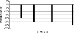
For simplicity, the width (b) of the rectangular cross section was defined as the design variable. Hence, the perturbations in the stiffness and mass matrices are linearly proportional to the structural variables. To generate a perturbed system, the widths of four elements 5, 10, 19, and 25 were reduced by 20, 25, 25, and 30% arbitrarily, as shown in .
Figure 2. Element modifications of perturbed system.
A finite element program was used to calculate the lowest five eigenvalues of the baseline and perturbed systems, as illustrated in . It should be noted that even the element changes of significant magnitude cause small perturbations in the modal responses, which indicate the low sensitivity of eigenvalue to element modifications.
Table 1. Eigenvalues of baseline and perturbed systems
The exact modal data (eigenvalues and primary degrees of freedom) of the perturbed system are applied for the inverse problem. The number of modes involved in the equation formulation will be increased from one up to five. In each mode, the inverse problem has 10 equations (primary degrees of freedom) for 25 unknown structural variables to be determined.
6.2. Selection of primary sets
The primary set includes the translational degrees of freedom of 10 nodes. shows the primary sets obtained from three selection criteria. Firstly, the sequential elimination of the secondary degrees of freedom with the smallest ratio of mii/kii yielded the primary set (A).
Figure 3. Selected primary sets.
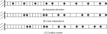
The left singular vectors obtained through singular value decomposition of the modal matrix ΦL were employed to get the primary nodes in set (B) for maximum linear independence. Through the use of Gershgorin's theorem, the primary set (C) was selected to obtain a transformation matrix of close distribution of eigenvalues and minimum condition number.
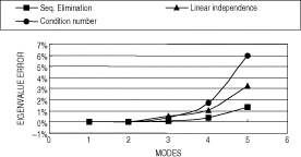
Convergence characteristics of the primary sets are illustrated in . The lowest eigenvalue of the secondary subspace λs dictates the rate of convergence in the infinite series expansion of the dynamic stiffness matrix. All the primary sets yielded the matrix ΦpL of rank five. A low condition number of S indicates the numerical stability of the transformation matrix in modal matrix projection. The minimum and maximum singular values of the modal matrix ΦL are 34.0144 and 48.0936. Hence, the condition number is obtained as μ(ΦL) = 1.9992.
Table 2. Convergence characteristics of selected primary sets
The selected primary sets were examined for the solution accuracy in static condensation. The percentage errors of the lowest five eigenvalues are illustrated in . The primary set (A) obtained through sequential elimination gives an excellent solution. It is interesting to note that the primary sets (B) and (C) selected for maximum linear independence and minimum condition number can show good accuracy in static condensation.
Figure 4. Solution errors in static condensation.
6.3. Exact transformations
The structural matrices and the modal data of the perturbed system were used to calculate the transformation matrices, which represented the exact relations between the primary and secondary degrees of freedom in system condensations. Then, the system reduction is the only source of solution error in inverse problems.
As more modes were added, the equation formulation became overdetermined and the inverse solution converged fast to the correct modification. Finally, the lowest five modes were employed to have 50 equations for 25 structural variables.
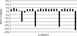
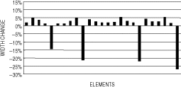
The application of the dynamic stiffness matrix for the system transformation of the primary set (A) gave the element changes in . The inverse solution would come a little short of the correct perturbations in . It is interesting to observe the constant small errors on the unperturbed elements.
Figure 5. Element identification with exact transformation (dynamic stiffness matrix).
On the other hand, the procedure of modal matrix projection yielded the structural modifications in . Nearly the same results were obtained with a slight decrease in the solution accuracy. It appears from the figures that the system reduction caused about 3–5% deviations in element identification, regardless of the method of system transformation. Primary sets (B) and (C) gave nearly the same results, which were omitted from the illustrations.
Figure 6. Element identification with exact transformation (modal matrix projection).
The reanalysis results of the inverse systems showed excellent eigenvalues, as shown in . Note that either of the transformation methods can provide a subspace eigenproblem to obtain an accurate inverse solution for frequency optimization.
Table 3. Eigenvalues with exact transformation
6.4. Inverse solutions
The convergence characteristics of inverse solutions were investigated while the number of modes increased from one up to five. The transformation matrices were updated in each iteration. For the termination criterion, the residual error was compared with the right-hand side of equation (57) and the tolerance was set to 10−6.
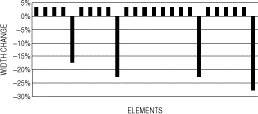
At first, the dynamic stiffness matrix was applied for the system transformation of the primary set (A). As the number of modes increased, the inverse problem became overdetermined and the solution converged to the correct modifications. With the lowest five modes involved, the inverse solution showed the element modifications in . As can be expected from , the constant deviations of about 3% were due to the system reduction error. Primary sets (B) and (C) showed the same tendency, which were omitted from the illustrations.
Figure 7. Inverse solution (dynamic stiffness matrix).
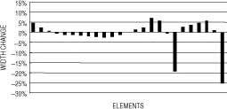
On the other hand, the procedure of modal matrix projection gave the inverse solution in , which was quite different from the approximation in . Also in this case, the lowest five modes were used in the equation formulations. Elements 19 and 25 at the outer section showed good agreements whereas the modifications of elements 5 and 10 had not come out at all. Contrary to expectations, the inclusion of higher modes had little effect on accelerating the solution convergence because of increasing errors in system transformations.
Figure 8. Inverse solution (modal matrix projection).
The inverse systems were analyzed to obtain the eigenvalues in . It is believed that both the dynamic stiffness matrix and the modal matrix can be used for the system transformation in structural optimization for frequency changes.
Table 4. Solution accuracy in eigenvalues
7. Conclusions
A modal method combined with system condensations proved to work well for inverse problems of linear dynamic structures. Through system condensations, the equilibrium equation of undamped free vibration was reduced into a subspace eigenproblem, in which a small set of degrees of freedom represented the corresponding eigenvector. Inverse solutions showed good convergence in frequency optimization. For element identifications, however, minor structural deviations were due to the system condensation error.
In the application of dynamic stiffness matrix, the solution convergence depends on the smallest eigenvalue in the subspace of the secondary structural matrices. The sequential elimination of secondary degrees of freedom yields the best primary sets. In large structures, however, the computational burden for repeated condensations should be attenuated through group-by-group eliminations.
The modal matrix of the baseline system can be used to project the measured data onto the perturbed mode shape. The primary modes obtained through sequential selection for maximum linear independence or minimum condition number showed good convergence characteristics not only in static condensation but also in inverse problems.
In structural optimization for frequency changes, excellent inverse solutions were obtained regardless of the selection of primary sets and the method of system transformations. For the inverse problem of structural identification, however, the application of dynamic stiffness matrix seems more suitable than the modal matrix projection.
Further research works will be conducted on the condensation of large structures and the consequent effect on the solution accuracy. In addition, the error propagation of the measured modal data or the numerical stability of the inverse solution is of great importance because dynamic measurements may have numerical errors from various sources.
Acknowledgement
This work was supported by INHA UNIVERSITY Research Grant, which is gratefully acknowledged.
References
- Leung, YT, 1978. An accurate method of dynamic condensation in structural analysis, Int. Journal of Numerical Method in Engineering 12 (11) (1978), pp. 1705–1715.
- Suarez, LE, and Singh, MP, 1992. Dynamic condensation method for structural eigenvalue analysis, AIAA Journal 30 (4) (1992), pp. 1046–1054.
- O’Callahan, J, Avitabile, P, and Riemer, R, System equivalent reduction expansion process (SEREP). Presented at Proceedings of the 7th International Modal Analysis Conference. Bethel, CT, 1989.
- Papadopoulos, M, and Garcia, E, 1996. Improvement in model reduction schemes using the system equivalent reduction expansion process, AIAA Journal 34 (10) (1996), pp. 2217–2219.
- Friswell, MI, Garvey, SD, and Penny, JET, Using iterated IRS model reduction techniques to calculate eigensolutions. Presented at Proceedings of the 15th International Modal Analysis Conference. Bethel, CT, 1997.
- Zhang, DW, and Li, S, Succession-level approximate reduction (SAR) technique for Structural dynamic model. Presented at Proceedings of the 13th International Modal Analysis Conference. Bethel, CT, 1995.
- Kim, KO, and Kang, MK, 2001. Convergence acceleration of iterative modal reduction methods, AIAA Journal 39 (1) (2001), pp. 134–140.
- Vanderplaats, GN, 1982. Structural optimization, AIAA Journal 20 (7) (1982), pp. 992–1000.
- Rao, SS, 1996. Engineering Optimization, Theory and Practice. New York: John Wiley & Sons; 1996.
- Kim, KO, Anderson, WJ, and Sandstrom, RE, 1983. Nonlinear inverse perturbation method in dynamic analysis, AIAA Journal 21 (9) (1983), pp. 1310–1316.
- Friswell, MI, and Mottershead, JE, 1995. Finite Element Model Updating in Structural Dynamics. Kluwer Academic Publishers; 1995.
- Moeller, PW, and Friberg, O, 1998. Updating large finite element models in structural dynamics, AIAA Journal 36 (10) (1998), pp. 1861–1868.
- Cherki, A, Lallenmand, B, Tison, T, and Level, P, 1999. Improvement of analytical model using uncertain test data, AIAA Journal 37 (4) (1999), pp. 489–495.
- Cobb, RG, and Liebst, BS, 1997. Sensor placement and structural damage identification from minimal sensor information, AIAA Journal 35 (2) (1997), pp. 369–374.
- Friswell, MI, Penny, JET, and Garvey, SD, 1997. Parameter subset selection in damage location, Inverse Problems in Engineering 5 (3) (1997), pp. 189–215.
- James, G, Zimmerman, D, and Cao, T, 1998. Development of a coupled approach for structural damage detection with incomplete measurements, AIAA Journal 36 (12) (1998), pp. 2209–2217.
- Berman, A, 1995. Multiple acceptable solutions in structural model, AIAA Journal 33 (5) (1995), pp. 924–927.
- Meirovitch, L, 2001. Fundamentals of Vibrations. McGraw-Hill; 2001.
- Friswell, MI, and Penny, JET, Is damage location using vibration measurements practical?. Presented at EUROMECH 365 International Workshop: DAMAS 97, Structural Damage Assessment using Advanced Signal Processing Procedures. Sheffield, UK, June/July, 1997.
- Kim, KO, Cho, JY, and Choi, YJ, 2004. Direct approach in inverse problems for dynamic systems, AIAA Journal 42 (8) (2004), pp. 1698–1704.
- Shah, VN, and Raymund, M, 1982. Analytical selection of masters for the reduced eigenvalue problem, International J. for Numerical Methods in Engineering 18 (1) (1982), pp. 89–98.
- Penny, JET, Friswell, MI, and Garvey, SD, 1994. Automatic choice of measurement locations for dynamic testing, AIAA Journal 32 (2) (1994), pp. 407–414.
- Kim, KO, and Choi, YJ, 2000. Energy method for selection of degrees of freedom in condensation, AIAA Journal 38 (7) (2000), pp. 1253–1259.
- Papadopoulos, M, and Garcia, E, 1998. Sensor placement methodologies for dynamic testing, AIAA Journal 36 (2) (1998), pp. 256–263.
- Strang, G, 1988. Linear Algebra and its Applications. Orlando: Saunders College Publishing; 1988.
- Golub, GH, and Van Loan, CF, 1996. Matrix Computations, . Baltimore: The John Hopkins University Press; 1996.
- Wilkinson, JH, 1965. The Algebraic Eigenvalue Problem. Oxford: Oxford University Press; 1965.
- Kim, KO, Yoo, HS, and Choi, YJ, Optimal sensor placements for dynamic testing of large structures. Presented at AIAA Paper 01–1232, 42nd SDM Conference. Seattle, WA, April, 2001.
- Kim, KO, and Anderson, WJ, 1984. Generalized dynamic reduction in finite element dynamic optimization, AIAA Journal 22 (11) (1984), pp. 1616–1617.
- Wilson, EL, Yuan, M-W, and Dickens, JM, 1982. Dynamic analysis by direct superposition of Ritz vectors, Earthquake Engineering and Structural Dynamics 10 (1982), pp. 813–821.
Appendix A: Singularities of submatrices
For a symmetric matrix A, a standard eigenproblem is written as
(------147296--59)
When the matrix of dimension n has rank L, the equation can be written in partitioned form as
(------147296--60)
The matrix A has rank-deficiency of order r (=n − L). The diagonal matrix ΛL contains the nonzero eigenvalues.
The equations for the zero eigenvalues can be separated as
(------147296--61)
The first equation of equation (A3) gives
(------147296--62)
It can easily be proved that ALL is singular if and only if Xrr is singular. In other words, ALL is nonsingular if Xrr is nonsingular.
Since the matrix A is symmetric, the modal matrix is orthonomal:
(------147296--63)
The equation for the off-diagonal terms gives
(------147296--64)
Hence, Xrr is singular if and only if XLL is singular. Therefore, both Xrr and ALL are nonsingular if XLL is nonsingular.