Abstract
This article deals with an inverse problem of determining source functions in an advection–dispersion equation under final observations. By using integral identity methods, a new approach which can be called data compatibility analysis methodology is presented and applied to solve the inverse source problem. By this method, the unknown is confined to an explicit admissible set which can be easily estimated through the compatible conditions. A real life example for determining magnitude of groundwater pollution sources in a actual geological region is investigated. An average magnitude of pollution sources here is obtained by the data compatibility analysis which also coincides with the results of numerical computations.
1. Introduction
With development of society and economics, groundwater pollution has become a serious threat to the environment. The government has to take some measures to prevent the groundwater from further contaminations. But the cost of cleanup for polluted aquifers is staggering, and in many cases it is hard to identify which companies are responsible for the contamination, due to lack of tools to discover the pollution sources. So, it is necessary to try to give more concrete information of the characteristics (location, magnitude, and duration of activity) of specific groundwater pollution sources (see Citation2,Citation5,Citation14).
As we know, most attempts at quantifying contaminant transport rely on mathematical methods. Since the data cannot be measured by direct ways in many cases, we are always encountering inverse problems of deciding unknown sources and aquifer parameters (see Citation12,Citation24 for instance). From the 1970s, there has been much research on such inverse and ill-posed problems in groundwater, and some wonderful results concerned with groundwater pollution source identification problems (see Citation6,Citation7,Citation15,Citation16,Citation18,Citation19, for instance). As stated by Atmadja and Bagtzouglou in a review paper (see Citation5), there are five classes of approaches in identification of groundwater pollution sources so far. The first class is using heat transport inversion methods because of the similarity in models of heat and mass transfer. The second class is applying optimization techniques sequentially employed by Gorelick, Evants, and Remson Citation13, Wagner Citation26, and Mahar and Datta Citation14,Citation16, etc. The third class is employing probabilistic and geostatistical simulation approaches, first utilized by Bagtzoglou Citation8, Bagtzoglou, Tompson, and Dougherty Citation9, and Bagtzoglou, Dougherty, and Tompson Citation10. The fourth class is based on either analytical solutions or nonlinear regression approaches presented by Sidauruk, Cheng, and Ouazar Citation17, and Ala and Domenico Citation1. The fifth class is using deterministic direct methods, proposed by Skaggs and Kabala Citation20–22, Birchwood Citation11, recently Atmadja Citation3, Atmadja and Bagtzouglou Citation4,Citation6, and Bagtzouglou and Atmadja Citation7, etc.
However, while a method is employed, it always encounters a theoretical problem that is stability criterion and non-uniqueness of the solution. For example, in identifying pollution sources via final observations, we always need to solve the governing equation backward in time, which is severely ill-posed. This kind of ill-posedness of inverse problems is essential, especially for real life problems. But a question in our mind is that if we can avoid solving governing equations, can we overcome the ill-posedness?
In this study, we will set forth a new approach to deal with such inverse problems of determining magnitude of groundwater pollution sources. Our basic model is solute transport equation, and additional data are the final observations of solute concentration. The methodology is based on compatibility analysis with aids of integral identities without solving the governing equations backward in time. By data compatibility analysis, known data are connected with unknown source terms, and the unknown term is confined to an explicit admissible set, and then it can be estimated easily. A real life example is investigated, in which the unknown source magnitude is estimated by data compatibilities. Furthermore, numerical computation with aids of MATLAB software is also carried out which perfectly supports the above theoretical results.
The article is organized as follows: in section 2, an inverse problem of deciding source magnitude in an advection–dispersion equation is put forward. Section 3 analyzes data compatibilities connecting known information with unknown terms, which plays a key role in the determination of the source term in this study. Section 4 is concerned with a real life example for determining magnitude of groundwater pollution sources in a geological region. Some characteristics of the source magnitude are discovered by applying the data compatibility analysis method in subsection 4.1, and a numerical computation as a testification for the same inverse problem here is performed in subsection 4.2, whose results roughly coincide with the theoretical analysis in subsection 4.1.
2. Inverse source problem
It is well-known that under suitable hypotheses, solute transportation in a homogeneous groundwater flow can be characterized via the following one-dimensional (1-D) advection–dispersion equation (see Citation25, for instance):
(------148498--1)
where, l > 0 denotes a bound for a studied region, T > 0 represents a final moment; c=c(x,t): concentration at time t and point x, dimension: M L−3; u: actual flow velocity of groundwater, dimension: L T−1; aL: longitudinal dispersivity, dimension: L; λ: attenuation coefficient, dimension: T −1; ne: effective porosity, no dimension; and q=q(x): average concentration of pollutants seeping into the aquifer per unit time, which represents the magnitude of pollution sources, dimension: M L−3T−1.
Now, let us consider initial boundary value conditions for equation (2.1).
First, the initial value is known as follows
(------148498--2)
Next, suppose the solute concentrations at the boundaries are known, that is to say we have the following Dirichlet boundary condition
(------148498--3)
Then, by equation (2.1), if the aquifer parameters and the seeping magnitude are all known, we can work out the concentration distribution c=c(x,t) by the initial boundary value conditions (2.2) and (2.3). However, the problem here is that the source magnitude function q=q(x) is unknown, which needs to be decided by some additional data. The additional data discussed in this study are observations at a final moment t = T given as follows:
(------148498--4)
Getting here, an inverse source problem is formulated, that is the problem (2.1–2.4), which is to decide the source magnitude q=q(x) with the over-posed condition (2.4).
3. Data compatibility analysis
Consider the inverse problem equations (2.1–2.4) again. For convenience, denote as the studied domain in the following discussions. Firstly, the unknown functions q=q(x) and c=c(x,t) are claimed to be positive for (x,t)∈ ΩT, and the data functions satisfy hypothesis (A) as follows
(A) c0(x), gi(t) (i=1,2) are all nonnegative, continuous, increasing functions.
Remark 1
This hypothesis is set to suit for a real life example investigated in section 4, and it is also necessary in the proof of the following theorems.
Next, suppose the parameters aL,u,λ, and ne satisfy an a priori hypothesis (B) as below
(B) .
In addition, the data should satisfy the following combining condition
(C) .
The following two theorems expose some compatible conditions on the data, which often lead to a definition of admissible set for the unknown functions.
THEOREM 3.1
Suppose c=c(x,t;q) satisfies an a priori bound estimate, the hypotheses (A), (B), and condition (C) are valid, and suppose further that q=q(x) has the following property
(D) .
Then it follows that
for (x,t)∈ ΩT.
Proof
For c=c(x,t;q) and any smooth test function ϕ (x,t), we have
Integration by parts leads to
(------148498--5)
Now, suppose ϕ =ϕ (x,t) solves the adjoint problem
(------148498--6)
Note that problem (3.2) imposes a condition on ϕ (x,t) at t = T, it is backward in time but is well-posed due to the reverse parabolic character of the partial differential equation.
If ϕ (x,t) solves (3.2), together with the initial boundary value conditions and hypotheses, equality (3.1) reduces to
(------148498--7)
where
In the following discussions, we are to prove that the sign of expression (3.3) is positive. Therefore, some reductions are needed for I2 and I3.
For I2, using integration by parts, and noting the boundary conditions, we have
Similarly, I3 can be reduced to
By virtue of the data compatibility (C), the expression (3.3) finally reduces to
Now, applying the maximum–minimum principle of parabolic type of PDE (see Citation23, for instance) to the adjoint problem (3.2), we conclude that if G(x, t) is nonnegative, but is otherwise arbitrary then ϕ (x,t) is negative in ΩT, and so does for ϕ (x,0). On the other hand, if ϕ (x,t)<0 in ΩT then combining with the boundary condition: ϕ (0,t)=ϕ (l,t)=0 of problem (3.2), imply that ϕx(0,t)<0 and ϕx(l,t)>0 for 0<t<T.
Hence, by virtue of the hypotheses (A) and (B), and noting that q having property (D), we know that the sign of (3.3) is positive.
Since G=G(x,t) is nonnegative but otherwise arbitrary, it follows that if there was any positive measure subset of ΩT where ct(x,t) was zero or negative, then a contradiction of (3.3) could be achieved by choosing the support G in this positive measure set. This proves that for each 0<x<l, there has ct(x,t)>0 for 0<t<T, i.e.
for (x,t)∈ ΩT. The proof is completed.▪
Now, let us introduce the following adjoint problem instead of (3.2)
(------148498--8)
where v(x) is a smooth, nonnegative input with decreasing property.
For this backward parabolic problem, set the unique input data v=v(x) belong to the following set:
Then, we have
LEMMA 3.2
The problem (3.4) has an unique nonnegative solution ϕ (x,t)∈ C2.1, and for some suitable v∈ V, there has .
Proof
First, by the transformation τ =T − t, the problem (3.4) can be reduced to an initial boundary value problem as follows
(------148498--9)
Second, since
, we have v(x)≥ 0. Then by the maximum–minimum principle as in Theorem 3.1, we know that the solution here takes nonnegative values. Moreover, noting that
, we can work out
for some suitable inputs v=v(x).
In fact, by variable separation method, the solution of problem (3.5) can be represented as follows
where
and
Therefore, we have
(------148498--10)
By the above expression (3.6), we know that in order to complete the proof, it only needs to estimate An. Fortunately, if setting the initial inputs v(x)=l − x, or
, then we can work out that
Thus, we have
together with (3.6) follows that the assertion is valid.▪
THEOREM 3.3
Under the conditions of Theorem 3.1, if furthermore, that the following properties are valid
(E) , and for 0<t<T, there has
(F)There exists
, satisfying
Then, we have
.
Remark 2
By the assertion of this Theorem 3.3, we know that for source magnitude function increasing on space, the final observations should also be monotone on the space.
Proof
Since
and with a similar method as used in the proof of Theorem 3.1, the above expression can be reduced to
(------148498--11)
where ϕ =ϕ (x,t) solves the adjoint problem (3.4). By Lemma 3.2, we know that if the sign of the two middle terms of the right-hand side of (3.7) is positive, then the assertion of
is valid.
In fact, by the properties (E) and (F), there exists ε > 0 such that
and
for 0<t<T*.
Therefore, noting to ϕ (l,t)<ϕ (0,t) in Lemma 3.2, we can work out that
By the above estimations, we finally get
which completes the proof.▪
According to the above discussions, an admissible set for the source functions can be defined as follows
That is to say, we should find the source function q within Sad. In the next section, by the above theoretical analysis, a real life example is investigated in which an average magnitude of groundwater pollution sources in a actual geological region can be easily determined via data compatibility restrictions.
4. A real life example
In this section, an acid pollution in groundwater in Fengshui, Zibo of Shandong Province, China is examined. The studied region is a relatively integrated unit of hydrologic geology whose area is about 45 km2. In this region, groundwater flow accumulated by atmosphere precipitation is gradually pressed when it seeps from the south-east to the north-west until it encountered the coal-seam, and so a strip containing rich groundwater is formed. By this reason, Yuedian and Zhanghua Wellspring were established in the 1980s. But with the excess exploitation of mines, e.g., the exploitation of coal-wells, groundwater pollution has become more and more serious in this region. In particular, acid contaminant of in Zhanghua Wellspring becomes higher and higher year after year. Our aim is to give a quantitative explanation to this phenomenon.
Therefore, the transport model of this acid solute is needed. Since the acid contaminant is of solubility, we assume it transforms slowly in the strip of saturated aquifer with completely soluble form. Together with the hydrologic geology condition in this region, we also assume that the aquifer is homogeneous, isotropic, and the dispersivity, attenuation coefficient, and effective porosity are all positive constants, and the retardation factor is equal to 1. Moreover, our attention is focused on 1-D transportation of the solute along the direction of groundwater flow.
Based on the above hypotheses, choosing the direction of groundwater flow which is from Sijiaofang to Zhanghau as the direction of X-axis, the acid solute transport in this groundwater system can just be characterized using equation (2.1). Now, let us consider the initial boundary value conditions.
Firstly, noting that the distance from Sijiaofang to Zhanghau is 4000 m, we take Sijiaofang as zero point, and l = 4000 (m). Next, let us regard 1988 as the initial year, 1999 as the final year, and then T = 11 (y). The following table gives some concentration values of in Sijiaofang and Zhanghua well-points from 1988 to 1999, which can be used to determine the initial boundary value conditions of this problem.
By the above actually measured data, we know that the pollution becomes more serious every year from Sijiaofang to Zhanghua, so the concentration should increase on time t, and the final observed data should also increase on space variable x.
Therefore, based on the above data listed in , we can get the following initial boundary value conditions by applying data fitting skills
(------148498--12)
Furthermore, by the similar technique, we can also get the solute concentration as additional data at the final year of T = 11 (y):
(------148498--13)
Table 1. Concentration data of  in the measured well-points.
4.1. Determining source magnitude by compatibility analysis
In this section, we will try to determine the source magnitude function q=q(x) in (2.1) by the above initial boundary value conditions and additional observations with the data compatibility analysis method. Therefore, we still need the model parameters that appeared in (2.1). Also by the actual hydrologic geology condition of the studied region and experiences, the parameters values are set as follows
Now, let us check the data compatibilities implied by Theorem 3.1 and 3.3, and then deduce some information for the unknown source function q.
First, the property (D) in Theorem 3.1 demands that q=q(x) satisfies the condition
by substituting into the actual data, we have
(------148498--14)
Next, by condition (E), we have q′(x)≥ 0, and
also by substituting into the actual data, we get
(------148498--15)
Finally, according to condition (F), noting that the range of the function
belongs to (4.145, 16.4199) as t∈ (0,11), there must be a time T*∈ (0,11) such that
as long as choosing
(------148498--16)
Thus, by the restricted conditions (4.3–4.5), we can give a cursory estimation for the unknown source magnitude q. For example, from (4.3), we know that the unknown source term could be a linear increasing function, which is greater that the function 0.00089375 x+7.0944. Next, from (4.4) we know that the left-hand source magnitude cannot be too small, whose average value could be about 3–4 (mg L−1). Finally, from (4.5) we can easily find that the right-hand source magnitude cannot be too strong, whose value should be confined to 16–17 (mg L−1). In summary, an average value of the source magnitude could be about 10–12 (mg L−1).
4.2. Testification by numerical computation
In this subsection with aids of MATLAB software, we will carry out a numerical computation to testify the theoretical result estimated in the above subsection.
Firstly, let us discrete the model (2.1). Take time step as τ, space step as h, and denote c(k, j) representing pollutant concentration at point (k, j). By Crank–Nicolson implicit difference scheme, we have
(------148498--17)
where
, and its coefficients are given below respectively
For convenience to compute, rewrite (4.6) as the following iteration form
(------148498--18)
where
Noting that the matrices M and N are both strict tridiagonal, it is stable and easy to solve equation (4.7) if the hydraulic parameters and source function are all known. Now, we will give a numerical computation for the source function q=q(x) with help of MATLAB. Therefore, also denote
, define an error functional as below
(------148498--19)
The inverse source problem here reduces to the following minimization problem:
(------148498--20)
So, we can work out the solution of problem (4.9) with MATLAB optimal function ‘fminsearch' by suitably choosing initial values of the source function q. In general, it is not easy to do such a thing. However, based on the above data compatibility analysis, a possible choice of initial values for the source term can be set to be in the range 10,12. The computation results are listed in . Where q0 denotes initial choice of the source magnitude, Err represents the computational relative error, and q denotes the fitting solution of the source magnitude.
Table 2. Source magnitude inversion by MATLAB function (h=100,τ =0.5).
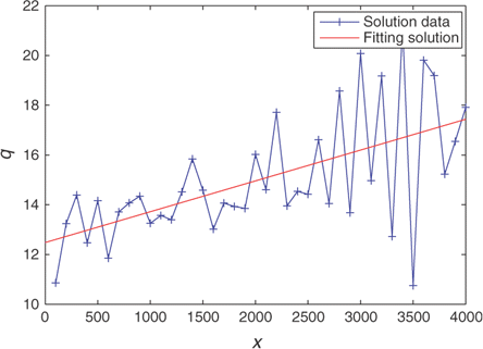
From the above computation results, we can observe that initial choice of the source magnitude is essential to the accuracy of the optimal research process. Fortunately, the minimal error appears as initial values of the source term belong to the domain of 14,16, and the corresponding source term solution is q(x)=0.0012x+12.48. Obviously, this fitting solution satisfies conditions (D), (E), and (F), and its average value is about 14.88 (mg L−1), which roughly coincides with the theoretical analysis by data compatibilities in the last subsection. Furthermore, taking this case as an example, the computational data of the source term solution and the fitting solution as q0∈ {14,16} are plotted in .
Figure 1. Computational solution data and fitting solution.
Remark 1
From the above discussions, we know that for the inverse problem of deciding magnitude of groundwater pollution sources investigated here, data compatibility analysis can lead to a very useful information for the numerical computation, and can give a preliminary estimate for the unknown.
Remark 2
For the numerical computation of the source magnitude q, a genetic algorithm is also applied to solve the minimization problem (4.9). A satisfactory result is that q(x)=0.000538 x+13.36, which can be regarded as another support for the method of data compatibility analysis used in this article.
Acknowledgments
Many thanks for the valuable suggestions of the reviewers and the Associate Editor. This work was supported by the National Natural Science Foundation of China (10471080), and Natural Science Foundation of Shandong Province (Y2001E03). The first author was also supported by the Visiting Funds from the Ministry of Education of China, and he thanks the Institute of Mathematics at Fudan University for its hospitality during his visit.
References
- Ala, NK, and Domenico, PA, 1992. Inverse analytical techniques applied to coincident contaminant distributions at Otis Air Force Base, Massachusetts., Ground Water 32 (1992), pp. 212–218.
- Alpay, ME, and Shor, MH, 2000. Model-based solution techniques for the source localization problem., IEEE Transactions on Control Systems Technology 8 (2000), pp. 895–904.
- Atmadja, J, 2001. "The marching-jury backward beam equation method and its application to backtracking non-reactive plumes in groundwater". Columbia University; 2001, Ph.D. Dissertation, 121.
- Atmadja, J, and Bagtzoglou, AC, 2000. "Groundwater pollution source identification using the backwack beam equation method". In: Computational Methods for Subsurface Flow and Transport. Rotterdam, The Netherlands: A.A. Balkema; 2000. pp. 397–404.
- Atmadja, J, and Bagtzoglou, AC, 2001. State of the art report on mathematical methods for groundwater pollution source identification., Environment Forensics 2 (2001), pp. 205–214.
- Atmadja, J, and Bagtzoglou, AC, 2001. Pollution source identification in heterogeneous porous media by MJBBE method., WRR 37 (2001), pp. 2113–2125.
- Atmadja, J, and Bagtzoglou, AC, 2003. Marching-jury backward beam equation and quasi-reversibility methods for hydrologic inversion: Application to contaminant plume spatial distribution recovery., WRR 39 (2003), pp. 1038–1047.
- Bagtzoglou, AC, 1990. "Particle-grid methods with application to reacting flows and reliable solute source identification". University of California Irvine; 1990, Ph.D. Dissertation, 246.
- Bagtzoglou, AC, Tompson, AFB, and Dougherty, DE, 1991. "Probabilistic simulation for reliable solute source identification in heterogeneous porous media". In: Water Resources Engineering Risk Assement. Vol. G29, NATO ASI Series. 1991. pp. 189–201.
- Bagtzoglou, AC, Dougherty, DE, and Tompson, AFB, 1992. Application of particle methods to reliable identification of groundwater pollution sources., Water Resources Management 6 (1992), pp. 15–23.
- Birchwood, RA, Identifying the location and release characteristics of a groundwater pollution source using spectral analysis. Presented at Proceedings of the 19th Annual American Geophysical Union Hydrology Days Conference. Fort Collins, Colorado, 1999.
- Constables, D, et al., 2002. Parameter identification by a single injection-extraction well., Inverse Problems 18 (2002), pp. 1605–1620.
- Gorelick, SM, Evans, BE, and Remson, I, 1983. Identifying sources of groundwater pollution: an optimization approach., Water Resources Research 19 (1983), pp. 779–790.
- Mahar, PS, and Datta, B, 1997. Optimal monitoring network and groundwater pollution source identification., Journal of Water Resources Planning and Management 123 (1997), pp. 199–207.
- Mahar, PS, and Datta, B, 2000. Identification of pollution sources in transient groundwater systems., Water Resources Management 14 (2000), pp. 209–227.
- Mahar, PS, and Datta, B, 2001. Optimal identification of groundwater pollution sources and parameter estimation., Journal of Water Resources Planning and Management 127 (2001), pp. 20–29.
- Sidauruk, P, Cheng, A, and Ouazar, D, 1998. Ground water contaminant source and transport parameter identification by correlation coefficient optimization., Ground Water 36 (1998), pp. 208–214.
- Singh, RM, Datta, B, and Jain, A, 2004. Identification of unknown groundwater pollution sources using artificial neutral networks., Journal of Water Resources Planning and Management 130 (2004), pp. 506–514.
- Singh, RM, and Datta, B, 2004. Groundwater pollution source identification and simultaneous parameter estimation using pattern marching by artificial neutral network., Environment Forensics 5 (2004), pp. 143–153.
- Skaggs, TH, and Kabala, ZJ, 1994. Recovering the release history of a groundwater contaminant., Water Resources Research 30 (1994), pp. 71–79.
- Skaggs, TH, and Kabala, ZJ, 1995. Recovering the history of a groundwater contaminant plume: Method of a quasi-reversibility., Water Resources Research 31 (1995), pp. 2669–2673.
- Skaggs, TH, and Kabala, ZJ, 1998. Limitations in recovering the history of a groundwater contaminant plume., Journal of Contaminant Hydrology 33 (1998), pp. 347–359.
- Sperb, RP, 1984. Maximum Principles and their Applications. New York: Academic; 1984.
- Sun, NZ, 1994. Inverse Problem in Groundwater Modeling. Dordrecht: Kluwer; 1994.
- Sun, NZ, 1996. Mathematical Model of Groundwater Pollution. New York: Springer; 1996.
- Wagner, BJ, 1992. Simultaneously parameter estimation and contaminant source characterization for coupled groundwater flow and contaminant transport modeling., Journal of Hydrology 135 (1992), pp. 275–303.