Optimization tools in the analysis of micro-textured lubricated devices

Abstract

We address the problem of optimizing the performance of lubricated devices by means of artificial texturing. We consider a slider (or equivalently a thrust bearing) and minimize the friction using optimization tools such as sensitivity analysis and genetic algorithms. We show that textures that perform significantly better than the smooth (untextured) one can be found, and that the optimized texture depends on the working conditions (load, velocity). The GENESIS code that we used, with no fine tuning of algorithmic variables, proved a valuable tool in the identification of improved shapes.

Keywords:

• Micro-texture
• Sensitivity analysis
• Optimization tools

Nomenclature

h	=	=Local film thickness
hp	=	=Depth of dimples
hmin	=	=Minimum film thickness
Ng	=	=Number of groups of dimples
ac	=	=Square cell side
ap	=	=Edgelength of the dimples
as	=	=Half distance between dimples
k	=	=Steepness parameter
x	=	=coordinate
y	=	=coordinate along film thickness
z	=	=coordinate
p	=	=Local pressure
U	=	=Velocity
W	=	=Load capacity
Wa	=	=Applied load
F	=	=Friction force

1. Introduction

Static and dynamic characteristics of lubricated devices are very sensitive to geometrical changes in the surfaces. The question then arises as to what improvements can be brought to, for example, a slider (which is also a model of a thrust bearing) by texturing its surface by some of the newly available methods such as indentation, chemical etching, laser ablation, etc. A few recent works have suggested that significant improvement can be brought to lubricated devices by artificial texturing 1–3.

This report addresses a preliminary study in this direction that makes use of optimization tools such as sensitivity analysis and genetic algorithms. We consider the simple case of a slider loaded with a static, vertical force. Only a texture on the static surface is considered, so that the texture distribution does not move with respect to the load and the problem has a time-independent steady state.

This simple case is important to understand the basic mechanisms that could bring improvement to the slider's performance. We study square texture cells with square microdimples, and optimize the dimples' size and depth.

The methodology is the solution of the Reynolds' equation by finite element method coupled to a Newton-like method to find the equilibrium position. At this position the relevant quantities, such as friction force and minimal film thickness, can be evaluated so as to drive the optimization algorithm.

The conclusions of this preliminary assessment are, basically, that optimization tools (either deterministic or stochastic ones) can indeed find improved designs of lubricated devices, even when the design variables are in fact at the micro-scale of the surface's texture. We considered it important to assess evolutionary algorithms because in some areas of tribology the current trend is towards very sophisticated shapes that are not parameterized variations of previous ones. This article reports on a first step towards a systematic treatment of “optimum tribological surfaces”, or “engineered tribological surfaces”, by means of evolutionary algorithms.

2. Theory and definitions

2.1. Governing equation

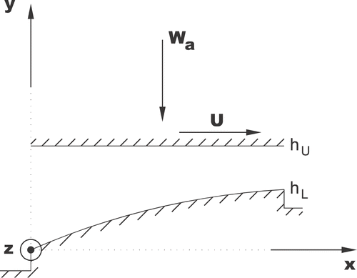
The basic relation governing the slider lubrication problem is obtained by introducing the Reynolds assumptions into the Navier--Stokes equation. This relation can be written in a non-dimensional form for the stationary case, in the (x, z) coordinate system (see figure 1) as: (1) where Ω is the integration domain and its boundary is defined as Ω = Γ _D\cup Γ N}, being Γ_D the Dirichlet part of the boundary and Γ_N the Neumann one.

Figure 1. Schematic view of a slider.

We consider two geometries. The first one is periodic in the width direction, and thus models a slider of infinite width, while the second one corresponds to a finite-width slider with atmospheric pressure along the sides. The corresponding boundary definitions are:

•	Infinite width
•	Ω = [qb;0,1]qb; ; × (- (ac/2(ac/2))
•	Γ _N = \{(x,z) \,|\, x ∈ [qb;0,1]qb; ; , z = \pm ({a_{\rm c}}/{2})\}
•	Finite width
•	Ω = [qb;0,1]qb; ; × [qb;Vh ;0, B]qb;Vh ;
•	Γ N = {(x,z) ,|, x ∈ [qb;0,1]qb; ;, z = (B/2)

where a_c is the square cell side and B is the slider width in the z direction.

The thickness of the fluid film can be expressed as: (2) where h_U is the height of the upper surface, in which the load is applied, h_L is the height of the lower (textured) surface, but omitting the texture contribution, and h_p is the contribution to the fluid film thickness coming from the texture (see figure 1). In the case considered here h_U is the following quadratic function: (3)

The equilibrium position h_U of the upper surface is found by Newton--Raphson iterations on the equilibrium condition (4) where W_a is the applied load, assumed along the y direction, and (5)

is the load capacity. The friction force F in the sliding direction (x) is calculated by integrating the shear stress along the fluid film: (6)

2.2. Dimples

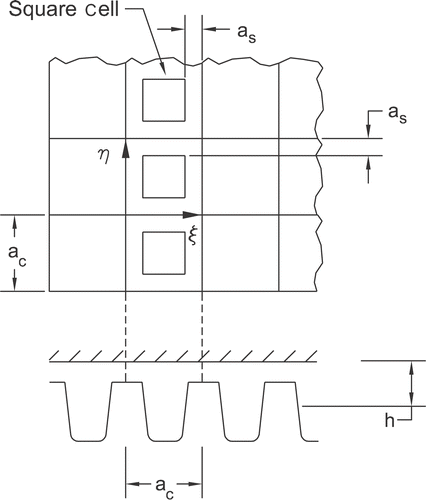
The dimples we consider are square and are arranged in a square pattern. They can be characterized by few parameters, as shown in figure 2. The edgelength of the square cell that contains the dimple is denoted by a_c. The edgelength of the dimple is a_p, so that the area fraction covered by dimples is simply . The third parameter that characterizes a dimple is h_po. In cell coordinates (ξ , η) the shape of the dimples is given by (7) where Ω _o = [V_h ;a_s,a_s+a_p}]V_h ;× [a_s,a_s+a_p], a _s = (1/2)\, (a_c-a_p) and k is a “steepness parameter”.

Figure 2. Schematic view of the dimples and an individual cell with its system of coordinates.

In the optimization process, the domain Ω is divided into regions. The dimples in each region are considered a “group” (N_g). The shape parameters (a_p, h_po and k) are varied keeping their values uniform for each group.

2.3. Numerical formulation

The numerical treatment of equation (1) is a quite standard Galerkin finite element formulation. Considering a discrete space V_h, which satisfies the Dirichlet conditions, one looks for a pressure field p_h∈V_h satisfying (8) where p_h- = min {p_h,0 }, and ε is the penalization parameter, that we take as 10^-10. The term involving ε models cavitation phenomena. In the limit ε → 0 it tends to satisfy the Elrod conditions p = ∂ p/∂ n = 0 at the boundary of the cavitation zone. The penalization is quadratic so as to render the left-hand side of (8) continuously differentiable with respect to p_h, which is convenient for the Newton--Raphson treatment of the nonlinearity. Though cavitation does not occur in the optimized shapes found in the cases reported here, it is important to include it because along the optimization process the evolutionary algorithms may propose shapes that produce cavitation.

2.4. Optimization -- genetic algorithm

Code GENESIS Version 5.0 of J. Grefenstette (http://www.aic.nrl.navy.mil/galist/src/#C) was used as the evolutionary algorithm in this study. A brief overview of the code is as follows:

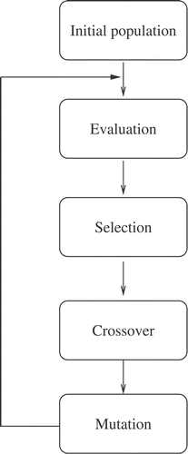
Let f:Rn → R be the objective function, and (X₁,X2, ··· ,X_n) its arguments (an n-vector). The algorithm works on a population (initially random) (9) making it evolve as shown in the diagram (see figure 3). Notice the classical steps in genetic algorithms 4:

•	Evaluation: Compute the objective function f. This is the most time-consuming step in our case since it involves a non-linear finite-element analysis.
•	Selection: Randomly choose those individuals that survive to the next generation, assigning more probability to those with smaller f.
•	Crossover: Randomly exchange genes (bits) between two individuals. The crossover rate can be controlled.
•	Mutation: Randomly invert bits of an individual. The mutation rate can be controlled.

Figure 3. Flow chart of the genetic algorithm.

The GENESIS code allows for the mentioned rates and the population size to be adjusted so as to have a reasonable convergence rate without saturation or instability.

3. Results and discussion

3.1. Rayleigh step -- test case

As first application a case with known optimum was chosen: The so-called Rayleigh step 5. In this problem the objective function is the load capacity. The problem reads:

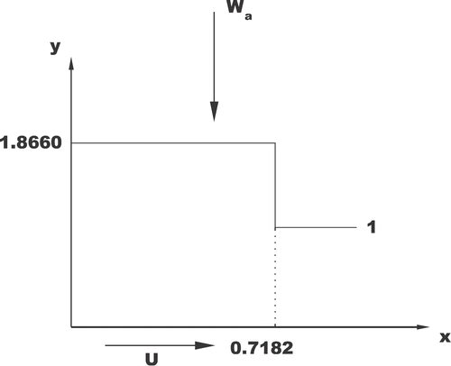
Find h*(x), h*(x) ≥ 1∀x ∈ [qb;0,1]qb; such that (10) where W[qb;h]qb; denotes the integral in (5) when p is the solution of (1). The exact optimum is given by (see figure 4): (11)

Figure 4. Non-dimensional Rayleigh step.

The code GENESIS was used in three different ways. Notice that in this “validation” problem there are no dimples; we are simply optimizing the shape h(x) in the set of piecewise constants.

In Case 1 the domain [qb;0,1]qb; ; was divided into 100 subregions, the value of h in each subregion being a state variable. The variation range for each variable was set to be the interval [qb;1,2]qb;.

In Case 2 the subdivision was the same, but the first 65 variables were assigned the range [qb;1.5,2]qb;, the following 10 variables the range [qb;1,2]qb; and the remaining 25 variables the range [qb;1,1.5]qb;.

Finally, in Case 3 it was assumed that the profile had stepped shape. The state variables were, thus, the film thickness on the left of the step, h_left, the film thickness on the right, h_right, and the discontinuity location, D.

The results from the first two cases after 30,000 evaluations of the objective function can be seen in figure 5, compared to the exact optimum. Results from Case 3 can be observed in table 1, as a function of the number of evaluations. The load value obtained for Case 1, corresponding to the shape shown in figure 5 is 0.9789 of the exact optimum, while that of Case 2 is 0.9921 of the exact optimum. In these cases a population size of 50 individuals was taken.

Figure 5. Results of the GENESIS code compared to the optimal Rayleigh step. Left: Case 1, Right: Case 2.

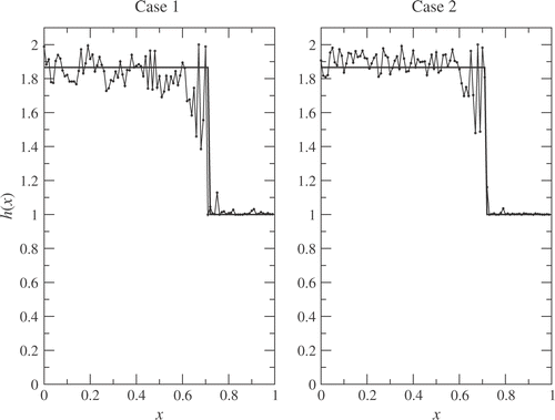
Table 1. Results of the GENESIS code compared to the exact ones, indicating the number of evaluations (Case 3).

Parameter	hleft	hright	D
Exact	1.8660	1	0.7182
100 Eval.	1.8756	1.00044	0.7029
500 Eval.	1.8662	1.00048	0.7029
4000 Eval.	1.8662	1.00039	0.7154
10,000 Eval.	1.8662	1	0.7174

The mutation and crossover rates used in the calculations were 0.001 and 0.6 respectively.

The above results show that in general the genetic algorithm leads to “rough” shapes, especially in regions where h is much greater than one. The lubrication equation is not very sensitive to changes in the film thickness at regions where this thickness is large. Since the “rough” shapes have loads very close to the optimal one, no driving force exists for smoothing out the shape. Of course, if the algorithm is allowed to proceed indefinitely, the exact shape is eventually attained. For Case 2 above this happens after 200,000 function evaluations, approximately, and only then the obtained shape is “smooth”. It could be interesting to design a smoothing procedure specific for partially optimized lubrication shapes. It has also been shown that adding information, as is expected, narrows the state space and allows the algorithm to get close to the optimum in fewer generations.

Another interesting point is the algorithm's behavior as a function of the number of state variables. In table 2 we show the best load value (relative to the optimal one) as attained after 30,000 evaluations of the cost function. Compare the results with different numbers of state variables N_var = 50, 100 and 200. It is clear that the fewer the state variables, the fewer the number of iterations to get to within some given tolerance from the optimum. In all three cases the ranges of the variables were set according to Case 2 described earlier.

Table 2. Relative load capacity obtained with the GENESIS code using 50, 100 and 200 variables to define the film thickness h.

Nvar	Relative load capacity
50	0.9991
100	0.9921
200	0.9629

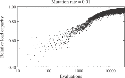
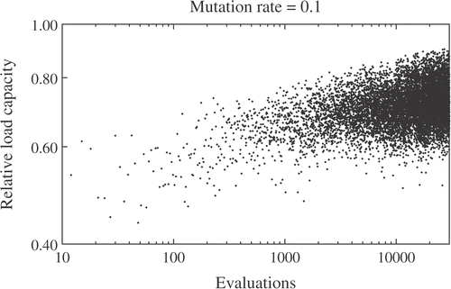
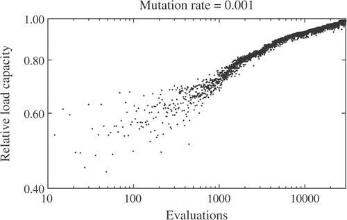
Finally, let us briefly comment about algorithmic parameters. The GENESIS code has default values for the crossover and mutation rate constants. Varying any of these constants does not have an impact on the convergence behavior of the algorithm. An example is shown in 6–8, in which the mutation rate constant is varied keeping the crossover rate constant fixed. It is observed that increasing the mutation rate constant by an order of magnitude does not affect practically the convergence behavior of the algorithm. Only after setting the constant to 100 times the default value (figures 8) does the mutation inhibit convergence.

Figure 6. History of the objective function along algorithmic iterations (relative to the exact optimum). The mutation rate constant is set to the default value of the GENESIS code, 0.001. The tics in the vertical axis have a spacing of 0.1.

Figure 7. History of the objective function along algorithmic iterations (relative to the exact optimum). The mutation rate constant is set to 0.01.

Figure 8. History of the objective function along algorithmic iterations (relative to the exact optimum). The mutation rate constant is set to 0.1, a value that is too high to attain convergence.

4. Textured sliders

Going now to the technological problem of texture design in the slider configuration (figure 1), in this case the objective function is f = F, the friction force, while the state variables {X_j} are texture-shape coefficients.

4.1. Infinite width case

We consider a square array of dimples, periodic in the width (z) direction. We first conducted a sensitivity analysis in order to narrow the search space, studying the variations of the friction and of the minimal spacing around the untextured state (h_po=0 everywhere) with respect to dimple depth.

Let denote the value of h_po for the Ith group of dimples. Since all other input data are fixed, the solution of the problem (i.e., the pressure field, the eccentricity, the minimal film thickness, the friction force, etc.) depends just on . We can thus calculate derivatives of any quantity, such as for example the friction force F, by numerical differentiation, that is (12)

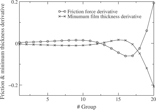
Whether it is convenient or not to carve dimples in some region of the bearing results from the derivative of F and h_min with respect to . These derivatives are shown in figure 9. Based on them, we consider the following dimple-depth distribution: (13) so as to allow dimples only where F is expected to decrease while h_min is expected to increase.

Figure 9. Friction force and minimum film thickness derivatives along the slider.

The dimple width is set to 1/100, and the domain is divided into N_g = 20 subregions, so that each subregion contains a group of 5 dimples. From criterion (15) the search space is narrowed to groups 12–17. In these groups we set as variables the dimple depth h_po, width a_s, and the steepness parameter k, within the ranges The total number of variables is thus 18.

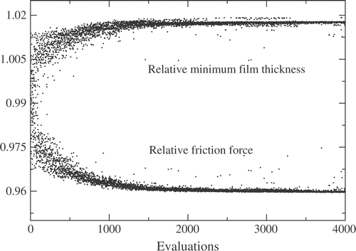
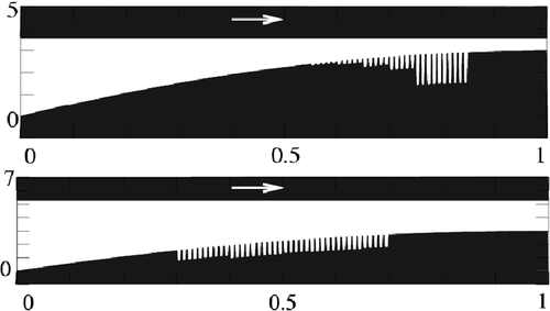
The evolution of the friction and of h_min along the evolution process is shown in figure 10 for a non-dimensional applied load of 0.06. Notice that the results are shown relative to the smooth case. A significant improvement of 4% is obtained. Moreover, this improvement comes with a 2% increase in the film thickness, which is important in terms of wear. The texture corresponding to the best individual found can be seen in figure 11. Also shown in the figure is the optimized shape corresponding to a smaller applied load, W = 0.006. It is clear that the optimized textures strongly depend on the operating conditions of the device.

Figure 10. Relative friction force and minimum film thickness. Evolution along the optimization process. Notice that a 4% decrease in friction, together with a 2% increase in minimum film thickness, is attained.

Figure 11. Optimized textures for two different non-dimensional loads: 0.06 (top) and 0.006 (bottom).

4.2. Finite width case

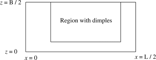
In this case we simulate half the width of the slider because of the symmetry. The cell width adopted is (1/24), so that the maximum number of dimples is 288 = 24× 12. Dimples are only allowed in the central portion of the slider (see figure 12), since from the previous paragraph we know that this portion is the one in which dimples can be beneficial.

Figure 12. Scheme showing the region in which dimples are introduced in the finite-width case.

In figure 13 we illustrate the pressure field corresponding to a uniform dimple depth of h_p = 0.5. The dimples were divided into 35 groups of 2× 2 dimples each. Two free parameters were assigned to each group of dimples, the depth and the size, with the ranges: h_po ∈ (0,1.3) - a _s ∈ [qb;0.0025,0.007]qb;.

Figure 13. Pressure distribution when a uniform texture is introduced in the region indicated in figure 12.

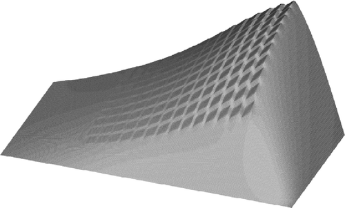
The total number of parameters is thus 70. Again the genetic algorithm found a design with a 4.7% reduction in friction force. The best texture found after 3000 evaluations of the objective function is shown in figure 14.

Figure 14. A 3D view of depth distribution of the optimized texture after 3000 evaluations of the objective function. The maximum depth is 1.292, the minimum one is 0.085.

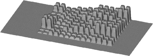
The result after 18,000 evaluations is given in figures 15 and figures 16. The reduction in friction force corresponding to this pseudo-optimal texture is 5.2/% .

Figure 15. Two 3D views of depth distribution of the optimized texture obtained after 18,000 evaluations of the objective function. The maximum depth is 1.294, the minimum one is 0.0025.

Figure 16. Optimized texture with the depth shown by means of color zones. The maximum depth is 1.294 (brighter), the minimum one is 0.0025 (darker).

5. Conclusions

The recent development of advanced surface texturing techniques, such as laser ablation, chemical etching, etc., opens the possibility of “engineered surfaces” for lubrication devices 2,3. There exists significant activity in this direction, since important gain can be achieved in terms of friction, wear and lifetime extension.

It should not, however, be believed that some magical texture exists that is optimal no matter what the load and velocity of the device is. For each specific working condition, there exists a specific texture that improves the performance, but it depends on the load and velocity. Optimal design is thus necessary to identify the surface shape that is best for each device. It is thus appropriate to assess different optimization tools in this problem.

In this article we have focused on evolutionary algorithms, which have the potential of identifying global optima, and the results have shown that quite standard genetic procedures work rather well for the problem under study. Further investigation is however required since the cases considered do not involve crucial phenomena such as massive cavitation and viscous heating.

Notice, to conclude, that we have assumed throughout this analysis that the Reynolds approximation holds. This requires that the length scales in the sliding direction are much greater than the dimple depth. If the dimple length is comparable to its depth, the Navier--Stokes equations need to be solved to calculate the effect of the dimples and eventually optimize the design. This is the subject of ongoing research.

Acknowledgement

The authors acknowledge support from Agencia Nacional de Promoción Científica y Tecnológica (Argentina) through grants PICT'99 12-6337 and PICT'00 12-9848.

References

- Ronen Etsion, A, Etsion, I., and Kligerman, Y, 2001. Friction-reducing surface-texturing in reciprocating automotive components., Tribol. Trans 44 (2001), pp. 359–366.
- Etsion, I, and Halperin, G, 2002. A laser surface textured hydrostatic mechanical seal, Tribol. Trans 45 (2002), pp. 430–434.
- Ryk, G, Kligermand, Y., and Etsion, I, 2002. Experimental investigation of laser surface texturing for reciprocating automotive components, Tribology Transactions 45 (2002), pp. 444–449.
- Pham, D.T, and Karaboga, D, 2000. Intelligent Optimization Techniques -- Genetic Algorithms Tabu Search Simulated Annealing and Neural Networks. Springer: London; 2000.
- Rayleigh, L, 1918. Notes on the theory of lubrication, Philosophical Magazine 35 (1918), pp. 1–12.