Abstract
In this article, we present an optimization model which incorporates uncertainty induced by geometrical imperfections. Within the model, geometrical imperfections are represented by means of random fields. The induced uncertainties are then treated using the concept of a convex model. The resultant problem is then solved in a two-stage optimization procedure. An arched girder is used to demonstrate the capabilities of the proposed approach.
1. Introduction
Today, optimization methods have proven to be a powerful tool for the design of complex structures in civil engineering. However, the performance of the optimized structure in real conditions depends essentially on the quality of the model used for optimization. This holds particularly for the optimization of slender structures subjected to compressive stresses. Using conventional models, optimization of this type of structures is prone to generate designs that are highly sensitive to geometrical imperfections Citation14. Therefore, it is crucial to develop an optimization methodology which leads to results which behave reliable within a specified range of imperfection shapes.
The subject of this article is an optimization model for slender structures under compressive loading. In distinction to a previous work, for example Citation9, the uncertain nature of geometrical imperfections is explicitly taken into account. Hereby, the treatment of uncertainties is similar to e.g. Citation12, Citation7, or Citation5 but the scope of application is extended to complex structures from the field of civil engineering that require advanced concepts of geometrical modeling.
In structural optimization the underlying design problem is formulated as a mathematical optimization problem. The scalar valued continuous optimization problem takes the form
(1)
where x is the n-dimensional design vector and f0 the objective function. The set S denotes the feasible domain and is defined by
(2)
The m functions f1,…,fm are called constraint functions and contain the requirements the structural design has to fulfill. In the following, the m + 1 functions f0,…,fm will be collectively called problem functions. Problem functions are set up by means of a computer based optimization model such that the relevant aspects of the design problem are covered. As noted earlier, for slender structures imperfections and stability behavior is a governing aspect. In the following, an appropriate optimization model is presented.
The next section deals with the elements and the general structure of the model. Then, the approach to the description of the imperfect geometry of the structure is presented. This includes the geometry to be optimized as well as a model of geometrical imperfections. The chosen approach to the treatment of the uncertainties induced by the imperfections is dealt with, subsequently. Finally, an arched girder as an example of a complex engineering structure is optimized.
2. Optimization model
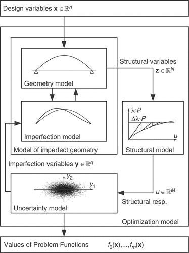
The developed optimization model consists of four interacting sub-models: (i) The geometry model realizes the dependency of the structural variables from the design vector . The possible deviations from the idealized geometry, as described by the imperfection vector
, are described in (ii) the imperfection model. Together these two form the model of the imperfect geometry which describes (iii) the analysis model by means of the structural variables
. In order to capture the stability behavior correctly a geometrical nonlinear analysis is necessary. Despite the uncertainties present in the model, unambiguous statements about the overall structural performance have to be made. This is done in the (iv) uncertainty model. Based upon the output of the uncertainty model, the values of the problem functions f0(x),…,fm(x) are computed. shows the overall model.
3. Geometry description
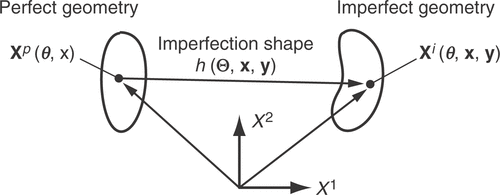
For the geometry model, a relation between the perfect and the imperfect geometry is needed. This relation is given by the imperfection shape h which assigns to each point of the perfect structure Xp a deviation as shown in .
The design of the geometry model has two goals: (i) an efficient representation of the structure by only a few optimization variables and (ii) the option to integrate an imperfection model.
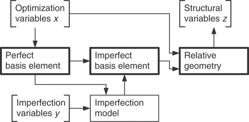
The starting point for the geometry model is a so-called basis element which represents the overall shape of the structure. This basis element is a curve for one-dimensional structures, like curved beams or arches, and a surface for two-dimensional structures like shells or grid shells. This basis element is represented by means of NURBS Citation8 which are widely used in computer aided geometric design. Along with the imperfection model, the imperfect basis element is defined which then serves as a reference frame for the definition of a so-called relative geometry. Finally, the relative geometry defines the coordinates of the finite element nodes. The described scheme is illustrated in and applied to one-dimensional structures in the next section.
3.1. One-dimensional structures
The basis element of one-dimensional structures is the system curve
(3)
which is marked as perfect by the superscript p. Hereby rp is a NURBS of which the control points and weights are linked to the according entries of the design vector x. For the sake of a compact notation, this dependency is not included in (Equation3
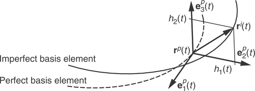
(3) ). A trihedron having the base vectors
,
and
and following the perfect basis element is defined. In the case of one-dimensional structures, the imperfection shape depends only on the curve parameter t and has two components:
(4)
Again, the dependency of h(t) from x and y is not explicitly noted.
In accordance to , the imperfect system curve yields to
(5)
Then again, a following trihedron is attached to the imperfect system curve. This trihedron serves as a reference frame for the relative geometry. Here, the remaining dimensions of the system are again described by NURBS. The final results are the curves on which the nodes of the finite element model are located.
The generalization of the concept to two dimensional systems (shells or grid shells) is straightforward and can e.g. be found in Citation1.
4. Geometrical imperfections
Geometrical imperfections can be interpreted as a phenomena of random nature. Nevertheless, the fluctuations at two different points are not completely independent, rather they are coupled stochastically over their distance.
For the modeling of such spatially varying random quantities the concept of random fields Citation15 is well suited. An application of random fields to geometrical imperfections is given in Citation11.
4.1. Scalar random fields
Within this article, the scope is on scalar valued random fields but an extension to vectorial random fields is straightforward.
A scalar random field H assigns to each point x within the considered domain a random number H(x). A realization h of the random field H is a function which assigns a number h(x) to each point x. Applying this concept, the properties of a random field can be stated.
4.1.1. Properties of random fields
In each point, a scalar random field has a distribution function
(6)
Moreover, the mean value function
(7)
gives the expected value of the random field at each point while the covariance function
(8)
captures the stochastic coupling of the fluctuations of two arbitrary points.
4.1.2. Modeling decisions
When random fields are employed to model real world phenomena, the properties introduced earlier have to be adequately identified. Usually, geometrical imperfections do not show a preferred direction and an accumulation around the perfect geometry has to be expected. Therefore, in this work the random field is Gaussian, having a mean value of zero. In addition, a homogenous correlation structure is used. This means that the value of the covariance function depends only on the relative position of two points. The covariance function thus depends on a scalar parameter ξ = ξ(x1,x2) which reflects the metric of the considered domain. Using such assumptions and an inverse exponential correlation function, the covariance function writes as
(9)
where σ is the standard deviation and b is called correlation length.
4.2. Discretization
For the implementation in a computer program, the above continuous formulation has to be discretized. For that, the random field is considered at discrete points. The original random field is then represented by a vector of random numbers
(10)
in which p is the number of discretization points. The covariance matrix of Z is computed by means of the covariance function (Equation8
(8) ) and is
Due to the symmetry of the covariance function, the covariance matrix is symmetric and, as can be easily shown, positive definite.
4.3. Constrained random fields
Often, it is necessary to take into account the constructive design of the system. For instance, in many cases one can ensure vanishing variances at the supports of a structure. In such a situation, the imperfection shape is represented by a new random vector
having an adapted covariance matrix. For Gaussian randomfields, this can be accomplished on the basis of a stochastic interpolation procedure Citation3. Let
be the points for which the variance is known to disappear. Then, using the matrices
and
the adapted covariance matrix yields to
(11)
shows qualitatively the covariance matrix of a linear one-dimensional random field. The left picture shows the original covariance matrix and the right picture the covariance matrix of the random field constrained at both ends.
4.4. Transformation in the uncorrelated space
As the covariance function (Equation9(9) ) takes positive values for each x∈D, the covariance matrix
has only nonzero entries such that the random vector
is fully correlated. For the treatment of the random field in the uncertainty model, it is necessary to represent the random vector
in terms of a new random vector Y which has more convenient properties.
Therefore, a set of base vectors a1,…,aq which are collected in the matrix is introduced. The random vector
is then represented by the linear combination
(12)
The covariance matrices of
and Y are connected by the set of base vectors A through the relation
(13)
which can be found by inserting the linear combination (Equation12
(12) ) in the well-known definition of covariance.
The next step is to choose the matrix A. This is done by applying a spectral decomposition on
. Since
is positive definite, it can be written as
(14)
where Q is the matrix formed by the eigenvectors qi of
and Λ is a diagonal matrix containing the corresponding eigenvalues. The comparison of (Equation13
(13) ) and (Equation14
(14) ) yields that, if
(15)
then BY is the identity matrix I. Thus, by employing the basis (Equation15
(15) ), the imperfection shape is represented by a linear combination of deterministic base vectors scaled by their probabilistic weights and uncorrelated uniformly distributed random numbers.
shows the first five base vectors for a one-dimensional random field of length one with σ = 1 and b = 0.5. The left picture corresponds to an unconstrained random field while the right picture shows the base vectors of a random field having a vanishing variability at both ends. It is clearly visible that the amplitude of the base vectors decreases as their variability increases.
5. Modeling of the uncertainty
The model of the geometrical imperfections presented introduces a substantial amount of uncertainty in the structure. Following Elishakoff Citation4, there exist mainly three approaches to handle uncertainty in structural analysis: (i) the classical probabilistic approach in which one aims for failure probabilities, (ii) the option to represent uncertain parameters as fuzzy sets, and (iii) convex models of uncertainty. In addition, the concept of fuzzy randomness introduced recently Citation6 is an approach which includes both probabilistic and fuzzy concepts.
Since the model of the geometrical imperfections has a probabilistic foundation, the fuzzy approach is not necessary. The probabilistic approach has the disadvantage of being potentially numerically expensive and requiring extensive knowledge of the stochastic properties of the uncertain parameters. The latter argument is particularly essential, because for the imperfections of complex structures it is difficult to aquire sufficient knowledge about probability distributions. For these reason, a convex model of geometrical imperfections based upon the above imperfection model is presented.
5.1. Convex modeling
The idea of convex models, which goes back to Ben-Haim and Elishakoff Citation2, is based upon the assumption of unknown but bounded uncertain parameters. For that, a subset of possible parameters Sy is defined which has the property of being convex.
The authoritative structural response vi(x) is then the worst structural response for all uncertain parameters contained in the set Sy. This condition is formulated as the optimization problem
(16)
which can be solved using existing optimization software. Since (Equation16
(16) ) denotes the search for the worst structural response, convex modeling is often associated with the term anti-optimization.
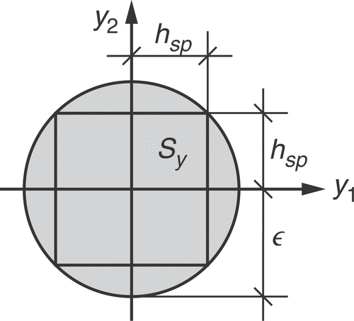
The next question is as how to choose the convex set Sy such that the original probabilistic properties of the random vector Y are appropriately captured. Since the entries of Y are normally distributed random numbers, the convex set has to be invariant against rotations of the coordinate system. This requirement is fulfilled by the set
(17)
which represents a q-dimensional ball. The radius ε of the ball is therefore the parameter governing this convex model. The basis for the parameter ε is the characteristic amplitude of the imperfection shape hsp.
The value hsp is chosen according to Citation13 from the 95% fractile of all imperfection shapes. According to , the radius then becomes
(18)
where q is the number of imperfection variables.
5.2. Formulation as an unconstrained problem
Due to the specific structure of the convex set (Equation17(17) ) it is possible to transform the constrained optimization problem (Equation16
(16) ) into an unconstrained one. This is carried out by means of a projection.
Using the new vector of imperfection variables
(19)
the projection
(20)
is defined. The domain of ψ is exactly Sy and
(21)
holds. In equation (Equation19
(19) ), the entry
can be interpreted as a slack variable, which allows the representation of interior points of Sy. Using the relation (Equation21
(21) ) and
the constrained anti-optimization problem (Equation16
(16) ) can be written as
(22)
which represents an unconstrained problem.
5.3. Derivatives
The optimization algorithms employed in this work need the derivatives of the problems functions with respect to the design variables. Consequently, the derivatives of the worst structural responses (Equation22(22) ) have to be computed.
Based upon the condition (Equation22(22) ), a functional dependency amongst
and x is formulated:
(23)
and the relation
(24)
can be stated. Using the chain rule of differentiation, the partial derivatives of (Equation24
(24) ) yields
(25)
On the other hand, the gradient
(26)
must vanish due to the necessary condition for the solution of problem (Equation22
(22) ). Therefore, using
*, the result
(27)
is obtained. This is crucial for two reasons: (i) the convex modeling, as performed here, does not influence the C1 continuity of the problem functions and (ii) the anti-optimization problem does not have to be solved in the perturbation steps of the numerical sensitivity analysis.
5.4. Algorithm
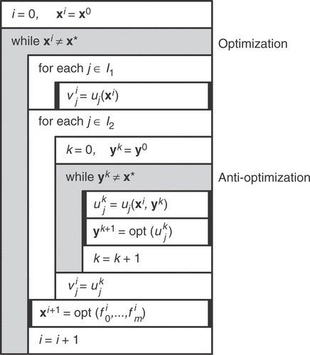
The solution of the overall optimization problem requires a procedure which comprises two nested optimization loops. In the outer loop, the optimization of structure is carried out. In the inner loop, the worst combination of the imperfection variables for the requested response quantity is determined.
In defining the solution algorithm, a distinction is required between response quantities which depend on the imperfection variables (e.g. stresses) and those which do not (e.g. weight). Let
(28)
denote the indices of response quantities independent of y and
(29)
those which depend on the imperfection shape.
The overall procedure is depicted in using a Nassi–Schneiderman notation. Obviously, the required computational effort depends mostly on the number of elements contained in the set I2.
6. Application example
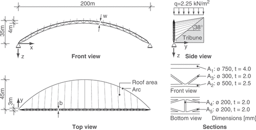
In this section, the optimization model described previously is applied exemplarily to an arched girder shown in subjected to a constant area load on the roof area. The material for the structure is steel, the modulus of elasticity is E = 2.1·105 N mm−2 and the density ρ = 7850 kg m−3. The structural model consists of 77 nodes and 209 truss elements having a circular cross section (tubes). The weight of the initial structure is 41.022 kg.
Geometrical imperfections are modeled by means of a random field. Since the structure is spatial, the random field implies two components, each of which is described by ten imperfection variables. The random field has an inverse exponential correlation function. At the two supports, no random deviations are assumed. The parameters of the imperfection model are collected in .
Table 1. Parameters of the imperfection model.
Within the geometry model, the structure is described by 21 optimization variables. Five optimization variables refer to the wall thicknesses of the cross sections and 16 variables describe the geometry of the structure. As the objective function, the strain energy stored in the deformed system is used. The optimization is subject to two constraints: (i) the weight of the structure must not exceed 41.300 kg and (ii) the total height of the system is restricted to 40 m.
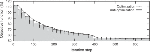
The optimization is carried out using the SQP algorithm Citation10. A comparison of the initial and the optimized structure is given in . Of special interest is the comparison of the strain energy for the perfect configuration (Perf.) and the worst imperfection shape (Imp.). Obviously, the increase in strain energy is much smaller for the optimized structure compared to the initial design. This is also visible in the optimization history shown in where the lower line belongs to the search for the worst imperfection shape carried out in each iteration step of the main optimization loop. The layout of the optimized structure is shown in .
Table 2. Objective function.
7. Conclusions
The optimization of structural systems with uncertainties induced by geometrical imperfections has been formulated. The presented model comprises a NURBS based geometry description, random fields for the modeling of geometrical imperfections, a nonlinear finite element analysis, and a convex model of uncertainty.
As an example of a complex engineering structure an arched girder has been optimized. The results achieved show that the proposed approach yields a structural design which is significantly less imperfection sensitive than the initial design.
| Nomenclature | ||
| = | design vector | |
| f0 | = | objective function |
| f1···fm | = | constraint functions |
| = | vector of imperfection variables | |
| h | = | imperfection shape |
| rp(t,x) | = | perfect system curve |
| ri(t,x,y) | = | imperfect system curve |
| [·, ·] | = | covariance of two random numbers |
| b | = | correlation length |
| BZ | = | covariance matrix of discretized random field |
| = | covariance matrix of discretized random field with constraints | |
| sy | = | convex set of allowed imperfection vectors |
| ui(x,y) | = | structural response quantity |
| vi(x) | = | structural response for controlling imperfection shape |
References
- Baitsch, M, 2003. Optimierung druckbeanspruchter Stabtragwerke unter Berücksichtigung geometrischer Imperfektionen. 2003, Dissertation, Institut für konstruktiven Ingenieurbau, Ruhr-Universität Bochum.
- Ben-Haim, Y, and Elishakoff, I, 1990. Convex Models of Uncertainty in Applied Mechanics. Amsterdam: Elsevier; 1990, Studies in Applied Mechanics.
- Dietlevsen, O, 1991. "Random field interpolation between point by point measured properties". In: Proceedings of the 1st Int. Conference on Computational Stochastic Mechanics. Corfu, Greece. 1991. pp. 801–812.
- Elishakoff, I, 1990. On the uncertainty triangle, Shock & Vibration Digest 22 (10) (1990), p. 1.
- Elseifi, A, Gürdal, MZ, and Nikolaidis, E, 1999. Convex and probabilistic models of uncertainties in geometric imperfections of stiffened composite panels, AIAA Journal 37 (4) (1999), pp. 468–474.
- Möller, B, Graf, W, and Beer, M, 2003. Safety assessment of structures in view of fuzzy randomness, Computers & Structures 81 (2003), pp. 1567–1582.
- Ohsaki, M, 2000. "Maximum loads of imperfect systems corresponding to stable bifurcation". In: Technical report. 2000, Architectural Information Systems Laboratory, Department of Architecture and Architectural Systems, Kyoto University. AIS Research Report No. 00-04.
- Piegl, L, and Tiller, W, 1995. The NURBS Book. Berlin: Springer; 1995.
- Reitinger, R, 1994. "Stabilität und Optimierung imperfektionsempfindlicher Tragwerke". In: PhD thesis. 1994, Institut für Baustatik, Universität Stuttgart.
- Schittkowski, K, 1985. NLPQL: a fortran subroutine solving constrained nonlinear programming problems, Annals of Operations Research 5 (6) (1985), pp. 485–500.
- Schorling, Y, 1997. Beitrag zur Stabilitätsuntersuchung von Strukturen mit räumlich korrelierten geometrischen Imperfektionen. 1997, Dissertation, Institut für Strukturmechanik, Bauhaus-Universität Weimar.
- Suzuki, K, and Ohtsubo, H, 1995. "The structural optimization under uncertainty". In: Computational Mechanics ’95, Theory and Applications, Proceedings of the International Conference on Computational Engineering Science. Hawaii. 1995.
- Thoft-Christiansen, P, and Baker, MJ, 1982. Structural Reliablility Theory and its Applications. Heidelberg, Berlin, New York: Springer-Verlag; 1982.
- Thompson, JMT, 1972. Optimization as a generator of structural instability, International Journal of Mechanical Sciences 14 (1972), pp. 627–629.
- Vanmarcke, E, 1983. Random Fields: Analysis and Synthesis. Cambridge, MA: The MIT Press; 1983.
