Evolutionary optimization using a new radial basis function network and the adjoint formulation

Abstract

This article aims at extending previously published ideas on the formulation and use of low-cost surrogate evaluation tools in the context of optimization methods based on evolutionary algorithms (EAs). Our goal is to minimize the cost of solving optimization problems with computationally expensive evaluations. A search algorithm is proposed which brings together computational fluid dynamics tools, namely flow and adjoint equation solvers, new radial basis function networks (RBFNs) and standard EAs. The new RBFNs involve additional control parameters which allow their training on patterns for which both responses and their gradients are available. In aerodynamic shape optimization problems, the gradient can be computed through the adjoint method. Despite the known role of adjoint methods, i.e. that of computing local search directions, in the proposed method they are used to enrich the available information for the training of the surrogate evaluation models, through providing the objective function gradient for each and every pattern. Based on a number of preselected samples, with known responses and gradients, the proposed RBFN is trained and used as the exclusive evaluation tool during the evolutionary search. A small number of cycles is required so as to capture the global optimal solution. A cycle includes the exact evaluation of the outcome of the evolutionary search, the RBFN update after retraining it on the enriched database, and a new search based on the updated RBFN. The method application is demonstrated through single- and multi-objective mathematical problems as well as the inverse design of a peripheral compressor cascade.

Keywords:

• Optimization
• RBFN
• EA

1.  Introduction

The computational cost of shape optimization methods is directly proportional to the number of candidate solutions that need to be evaluated before reaching the optimal solution. The larger number of required evaluations is the main drawback of evolutionary optimization methods and the main obstacle for their widespread use by the industry, especially if the evaluation of candidate solutions relies on the numerical solution of partial differential equations, such as the Navier–Stokes ones. To alleviate this problem, surrogate evaluation models can be used; in the past, several relevant algorithms have been proposed by our research group 1–4. In these works, various surrogate evaluation models (multilayer perceptron, RBFNs, kriging model) have been incorporated into evolutionary algorithms (EAs) and used as low-cost, surrogate evaluation models. Their role was to exploit previously evaluated solutions and, through them, approximate the fitness of new individuals.

Local surrogate models are those built and used only over parts of the search space. A local model is often associated with the neighborhood of a new individual and should be trained on the closest training patterns. Using local surrogate models, efficient EAs have been devised (see previously cited papers) selectively based on approximate or exact evaluation tools. A well-performing algorithm is the one based on the so-called inexact pre-evaluation (IPE) phase 5–7. IPE stands for an intercalary task used to pre-screen each generation's members; only the most promising among them are allowed to undergo exact evaluations. The cost for training local surrogate models is very small, so it can be assumed that the cost per generation is only that of exactly evaluating the topmost individuals. Thus, we prevent a great number of non-promising population members from being exactly evaluated and the total computational (CPU) cost is kept low.

In contrast, a surrogate evaluation model is considered to be a global one 8,9, if it is valid over the entire search space. The same global model can be used during the evolution to provide the “optimal” solution. The EA-based search which utilizes exclusively the (separately trained) global model has a negligible computing cost, in the sense that the cost of a single evaluation is almost zero. However, this “optimal” cannot be accepted without being re-evaluated through the exact tool. Depending on the deviation between its exact and approximate fitness values, a new EA-based search (cycle) may be necessary. Each new cycle makes use of an updated surrogate model, trained on a database enriched by the evaluated “optimal” solutions. Additional evaluated individuals at less-populated search space areas could also be added to the database, whenever deemed necessary.

Although the search through EAs assisted by surrogate models leads to a considerable economy of CPU cost, gradient-based optimization algorithms usually outperform EAs in terms of convergence speed. In CFD problems, control theory is employed to derive the adjoint to the flow equations whose solution provides the objective function gradient 10–12. This can be used along with any descent-like algorithm to get the optimal solution. However, depending on the initial solution, such a deterministic method may lead to local instead of global optimal solutions.

The algorithm proposed in this article merges the adjoint method (for the computation of the objective function gradient) and the use of global surrogate evaluation models (new RBFNs, with the additional capability of being trained on both responses and gradients) in an enhanced search method. There are only a few papers in the literature which report procedures for training surrogate models (artificial neural networks or response surfaces) using the gradient information 13–15. Using the new RBFNs, the EA undertakes the search of the optimal solution with almost negligible cost. As previously described, a few cycles are necessary. The proposed search algorithm and its constituent elements, one by one, are analyzed and tested in a number of mathematical and real-world problems.

The structure of this article is as follows: In the next section, the adjoint method is described in brief. Then, the new RBFNs are described in detail and a preliminary test, based on a univariate function interpolation, is shown. The presentation of the overall optimization algorithm follows. In the last section, single- and multi-objective problems are solved using the proposed method.

2. Gradient computation in flow problems – the adjoint method

The discrete adjoint method is used to compute the objective function gradient in 3D inverse design flow problems. Only inviscid flow problems are considered. The target is to design a 3D blade shape which yields a known (target) pressure distribution p_t over its surface S_w. The corresponding objective function I is defined by (1)

where p stands for the pressure field over the actual blade shape. Along with the minimization of the objective function I, the Euler equation (2)

should also be satisfied. Here, stands for the conservative flow variables' vector, while , , and are the convection fluxes. Equation (2) is numerically integrated over finite volumes centered at the nodes of a structured grid. An upwind scheme based on the Roe's approximate Riemann solver 16 with second-order variables' extrapolation is employed. Let us denote by the discretized flow equations. Also, let denote the design variables' vector which, in aerodynamic shape optimization problems, consists of the geometrical parameters defining the shape. The gradient of I with respect to the design variables reads (3)

Equation (3) is augmented by the product of the discretized flow equations gradient (4)

and the Lagrange multipliers . It, thus, yields the gradient of the augmented objective function (5)

By formulating and solving the discrete adjoint equations (6)

the terms remaining in equation (5) give the required objective function gradient (7)

Given the shape parameterization, the first term on the right-head side (r.h.s.) of equation (7) takes on analytically computed values. The second term, however, is computed through the central finite-difference formula which requires the repetitive computation of the residuals of the flow equations discretized around slightly (± ϵ , ϵ <<) bifurcated shapes.

3. RBFNs trained on responses and gradients

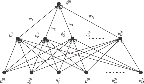
A typical RBFN which can be used in problems with N design variables () to approximate the single output , is illustrated in figure 1. The hidden layer should consist of N hidden units with synaptic weights w_i, i=1,N associated with the links between them and the output unit. In order to exactly interpolate the N input–output training pairs, each hidden unit is associated with the so-called RBF center , where .

Figure 1. RBFN with a single output unit.

The response ζ^(t) of a Gaussian function based RBFN (17, figure 1), is given by (8)

where is the Euclidean norm (9)

Unlike conventional RBFNs, where the weights w_i, i=1,N are the unknown quantities, computed by solving a linear system of equations with symmetrical coefficient matrix, here it is proposed to express w's in terms of two other families of unknown coefficients, namely β_i, i=1,N and α _i,m , i=1,N, m=1,M, as follows (10)

According to equations 8–10, the components of the RBFN response gradient are given by (11)

For N training patterns, N(M+1) conditions (12) (13)

should be satisfied. Through them, the βi, i=1,N and α_i,m,n=1,N, m=1,M coefficients are computed, by formulating and solving a linear system of equations.

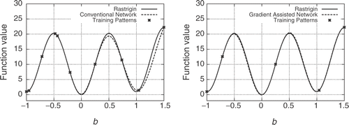
Before using the new RBFN in optimization problems, a first comparison between this and a conventional RBFN, in terms of their prediction abilities, is demonstrated. For the sake of fairness, the cost for collecting the training samples in either case should be equal. We recall that our target is to employ the RBFN-based search in design-optimization problems in fluid mechanics, in which the gradient is computed by the adjoint method with CPU cost approximately equal to that of performing a direct evaluation. In view of the aforesaid, a fair and meaningful comparison should use K (K may take on any integer value) training patterns for the conventional RBFN and only K / 2 for the new RBFN should be used. In figure 2, an easy-to-plot, multimodal, univariate function is plotted. From this figure, it is clear that the new RBFN performs a much more accurate interpolation with the same cost (see figure caption for more details). Thus, it seems to be better to utilize the new RBFN trained on half of the otherwise needed patterns with known responses and gradients.

Figure 2. Univariate function interpolation using conventional and new RBFNs. Ten (for the conventional RBFN, left) and five (for the new RBFN, with known gradient too, right) training points (b,τ ), where τ (b)= b² + 10(1- cos ( 2 π b)), have been used. After training the two RBFNs, the interpolated function is plotted along with the target–function curve.

4. The overall search method

The steps of the proposed single-objective optimization algorithm are described below:

Step 1:

The starting training dataset for the surrogate model is created. The training patterns can be defined using any Design of Experiment (DoE, 18) technique aiming at a well-representative sampling over the search space with the minimum number of samples. Regular grids, random sampling, (full or fractional) factorial designs, orthogonal arrays etc. can be used. In this study, the training patterns are chosen at random under some simple distance-based constraints.

Step 2:

For the previously selected individuals, the flow solver and the adjoint equations are solved. The so-computed responses and derivatives are stored in the database.

Step 3:

The surrogate model (RBFN) is trained; as explained in the previous paragraph, this step requires the solution of a linear system of equations, to compute the α and β coefficients.

Step 4:

The EA is used to obtain the “optimal” solution, using only the surrogate evaluation model.

Step 5:

The “optimal” solution is re-evaluated separately, using the exact evaluation tool. If the deviation between its approximate and exact fitness is less than a user-defined threshold, the algorithm terminates here.

Step 6:

The training set is re-defined by adding new entries or eliminating some of the existing ones. The most recent “optimal” solution, evaluated at step 5, is added to the training set; often, the closest to the “optimal” solution training pattern should be eliminated if the distance (nondimensional, measured in the parametric space) between them is less than a user-defined value. Optionally, κ new training patterns (κ is a user-defined small integer) can be added to the database after being exactly evaluated; these can be selected by running κ minor optimization problems, seeking for points with maximum average distance from the existing training patterns. This search can also be carried out by an EA and its computing cost is negligible. Windowing, i.e. the reduction of the search space is often beneficial to search (though optional) and, in this case, some database points can be eliminated from the new training set. Return to step 2.

With some modifications, the same algorithm applies to multi-objective problems as well. In this case, instead of adapting the search space (Step 6) around a single “optimal” solution, a more complicated algorithm is used to carry out the adaptation around the Pareto front members. A thinning process is used to reduce the number of entries in the Pareto front and control the number of additional entries into the training database.

5. Results and discussion

The algorithm proposed in this article is first applied to single- and multi-objective mathematical minimization problems in order to demonstrate its ability to locate either global optima or Pareto fronts. The new RBFN is compared with conventional RBFNs, trained solely on the responses of the objective function. Due to the simplified assumption that the costs of numerically solving the flow and the adjoint equations are almost equal, the conventional RBFN is always trained on twice as many as the samples used to train the new network.

5.1. The single-objective Ackley function

The first mathematical problem is the minimization of the Ackley function with M free parameters, defined by (14)

For visualization purposes, the first study is carried out using only two parameters (M=2), bounded in [-1, 1.5]. The global minimum (0,0) was known in advance and the search space was made asymmetric around this point.

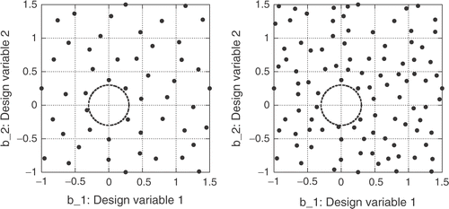
The initial training set for the new RBFN consists of 50 patterns, i.e. half of the patterns (100) used to train the conventional RBFN. In both cases, none of the sample points is allowed to lie within a circle with radius R = 0.3 around (0,0). The initial training patterns are selected at random, by taking care to prevent any two points from being located “next” to each other. The minimum distance is equal to 0.35 for the proposed network and 0.25 for the conventional one. The training patterns together with the point-free circle are shown in figure 3, for both networks.

Figure 3. Two parameter (M = 2) Ackley function: distribution of the N = 50 (new RBFN, left) and N = 100 (conventional RBFN, right) randomly chosen training patterns and the point-free circle around the optimal solution.

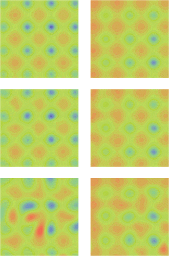
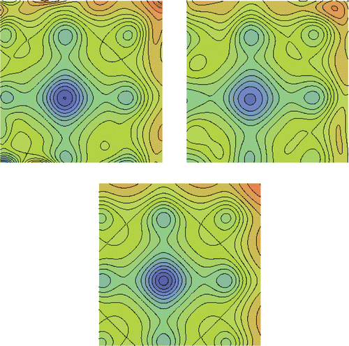
The optimization algorithm, based on the proposed RBFN  converges to the global optimum within two cycles. This quite fast convergence is explained in figure 4, in which the function iso-area contours reproduced by the two RBFNs (conventional and new) are compared with that of the exact mathematical function. The new network provides a much more accurate representation, though it was trained on half of the patterns.

Figure 4. Two parameter (M = 2) Ackley function: Iso-area contours: (a) predicted by the new RBFN (top-left), (b) predicted by the conventional RBFN, i.e. without taking into account gradient information (top-right), and (c) analytically computed (bottom).

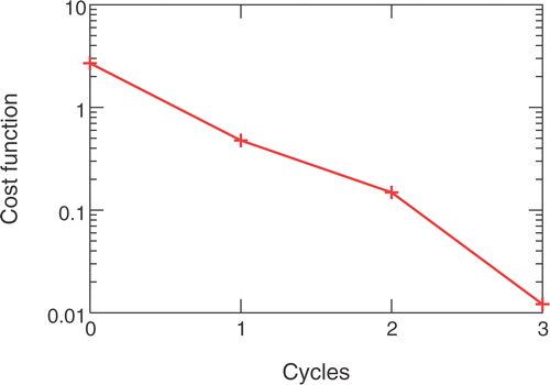
In order to show the ability of the proposed algorithm to handle problems with more design variables, it is applied to the same function, equation (14), with M = 10. The initial training set consists of N = 100 randomly selected patterns for conventional RBFNs and N = 50 for the new RBFNs. The response hypersurface in this case cannot be represented due to the dimensionality (10D). However, the optimization procedure reveals the ability of the new network to capture the minimum through just a small number of cycles. In particular, a convergence of about three orders of magnitude is obtained after four optimization cycles, see figure 5.

Figure 5. Ten parameter (M = 10) Ackley function: convergence history.

5.2. Two-objective function minimization problem

The second problem involves two mathematical functions with M = 2 degrees of freedom each. Both should be minimized, leading thus to the Pareto front of optimal solutions. The two functions are (15) where a₁ = 0, a₂=1.5, b1 ∈ [-2.12,1.12], and b₂ ∈ [-1.12,2.12].

The initial training set is formed by N = 50 randomly selected patterns for the training of the new RBFN (100 patterns for the conventional network), the same for each objective function. By the end of each cycle, the Pareto optimal solutions are exactly evaluated and added to the training dataset. In order to avoid unnecessary computational burden, which might occur whenever the Pareto front is overcrowded, a thinning technique is employed. The role of front thinning is to identify and keep a subset of the Pareto members (its size is user-defined), based on distance considerations.

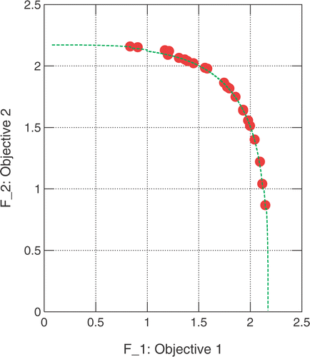
At the end of the optimization process the training dataset consists of 133 patterns. The final Pareto front computed using the proposed algorithm is compared to the exact front, figure 6. The response surfaces predicted by the proposed and the conventional RBFN and the exact response surface, over the nodal points of a dense grid, are shown in figure 7. The new RBFN performs better than the conventional one, in particular with respect to the first function.

Figure 6. Two-objective function minimization: The exact Pareto front (dashed line) and that computed using the RBFN (marks).

Figure 7. Two-objective function minimization: Response surfaces for the first (left column) and second (right column) objective functions. The exact shapes (top), the ones computed using the new RBFN (mid) and those produced using a conventional RBFN (bottom) are shown.

5.3. Inverse design of a 3D peripheral cascade

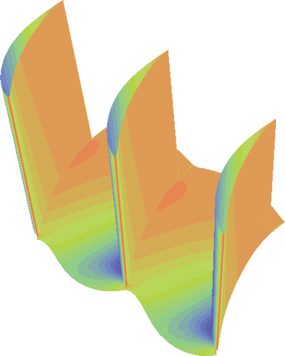
The last case is concerned with the inverse design of a 3D peripheral compressor cascade, with 41 blades. The flow conditions are M_out,is=0.4, a_in,per= 48° and a_in,rad= 0°. The flow (Euler) and the adjoint equations are solved on a structured grid. For an existing blade shape (reference geometry), the Mach number distribution which corresponds to the target-pressure one, is shown in figure 8.

Figure 8. Inverse design of a 3D peripheral compressor cascade: Mach number distribution over the reference cascade which corresponds to the pressure distribution imposed as target.

Each blade side is parameterized using (11 × 5) Bezier control points in the axial and radial directions. The peripheral coordinates of ten of them are allowed to vary; these correspond to the midspan blade section and also determine the other spanwise blade sections through a geometrical transformation.

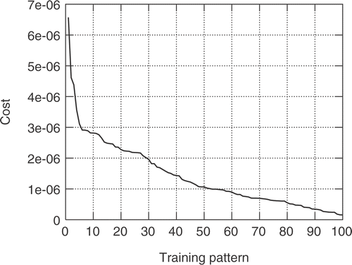
The initial training is made of 100 randomly selected training patterns. No patterns are selected within a small region centered at the global optimum. After being evaluated (by solving the flow and adjoint equations), the objective function value for each one of them is computed. This stands for the deviation between the target and actual pressure distributions, integrated over the blade surface. For the starting training patterns, these values (sorted in descending order) are shown in figure 9.

Figure 9. Inverse design of a 3D peripheral compressor cascade: Objective function value for the initial training patterns, sorted in descending order.

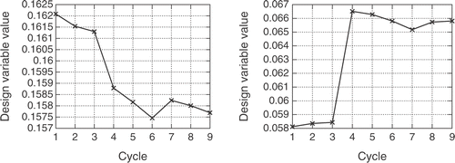
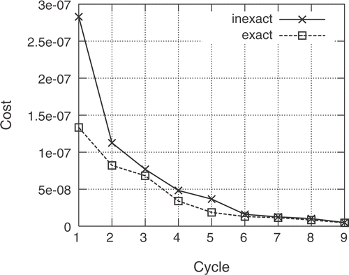
The CPU cost of the numerical solution of the flow and adjoint equations is about 4 min for each one of them, making thus a total CPU cost of about 13 h for the database formation. In each cycle, an optimization procedure takes place with the exclusive use of the RBFN as evaluation tool. The “optimal” solution found is separately evaluated using the direct and adjoint solver and is added to the training set. The network is retrained upon the enriched dataset and the algorithm ends when a convergence threshold is met. Nine cycles are required for convergence. In figure 10, the exact and approximate objective function values of the optimal “solution” of each cycle are plotted; each “optimal” solution was evaluated through both the flow solver and the RBFN. The convergence history for two selected design variables, during the nine optimization cycles, is shown in figure 11. It can be observed that, in the third cycle, the values for both shown variables changed considerably, underlying the ability of the method to escape from local optima. The iterative algorithm has converged about two orders of magnitude and the optimal Mach number distribution is almost identical to the one shown in figure 8 for the reference geometry. The total computational cost was that for evaluating (computation of response and gradient) the 109 blade geometries.

Figure 10. Inverse design of a 3D peripheral compressor cascade: Convergence history. The CPU cost associated with each cycle is that of a single evaluation (numerical solution of the flow and adjoint equations, i.e. two equivalent flow solutions) since the cost of retraining the RBFN and searching through EAs is almost negligible. The major burden is that of evaluating the starting training database (100 points in the search space, i.e. 200 equivalent flow solutions), not included in this figure.

Figure 11. Inverse design of a 3D peripheral compressor cascade: Monitoring of the second and sixth design variable values during the nine optimization cycles.

6. Conclusions

The adjoint method which is able to compute the objective function gradient in flow problems with reasonable CPU cost regardless of the number of the design variables, along with a modified RBFN which can be trained on both responses and gradients, are the major constituent tools of the optimization method presented in this article.

The proposed optimization algorithm utilizes an evolutionary method as search tool. During the evolution, a global surrogate evaluation tool is used. The computational cost is almost exclusively that of evaluating the initial training patterns and re-evaluating “optimal” solutions which come up during the repetitive evolutionary search. Despite the fact that the new RBFNs are trained on both responses and gradient, through the solution of a N(M+1) × N(M+1) system of linear equations, (N training patterns with M components each), the cost for training a well-performing network is low; in the examined compressor inverse design problem, it was about an order of magnitude less than that of solving the flow equations. However, direct solvers (like the one used herein) might become time-consuming if the problem size increases considerably (many design variables, M>>, and/or many training patterns, N>>), in which case an iterative solver could be used instead.

The new network is compared and proved to be more efficient than the traditional network which is trained solely on responses. Through a number of test problems, it was shown that the new network performed very satisfactorily both in mathematical single- and multi-objective minimization problems and the inverse design of a 3D peripheral cascade.

Acknowledgment

Support from the Research program Iraklitos, funded by the Greek Ministry of Education, is acknowledged.

References

- Giotis, AP, and Giannakoglou, KC, 1999. "Single- and multi-objective airfoil design using genetic algorithms and artificial intelligence, EUROGEN 99". In: Miettinen, K, et al., eds. Evolutionary Algorithms in Engineering and Computer Science. Jyvaskyla, Finland: John Wiley & Sons; 1999.
- Giotis, AP, Giannakoglou, KC, and Periaux, P, 2000. "A reduced cost multi-objective optimization method based on the Pareto front technique, neural networks and PVM, ECCOMAS 2000". Barcelona: CIMNE; 2000.
- Karakasis, M, Giotis, AP, and Giannakoglou, KC, 2003. Inexact information aided, low-cost, distributed genetic algorithms for aerodynamic shape optimization., International Journal for Numerical Methods in Fluids 43 (2003), pp. 1149–1166.
- Giannakoglou, KC, 2002. Design of optimal aerodynamic shapes using stochastic optimization methods and computational intelligence., Progress in Aerospace Sciences 38 (2002), pp. 43–76.
- Giotis, AP, Emmerich, M, Naujoks, B, Giannakoglou, KC, and Back, T, 2000. "Evolutionary Methods for Design, Optimisation and Control with Applications to Industrial Problems". In: Giannakoglou, K, et al., eds. Athens, Greece: CIMNE; 2000.
- Giannakoglou, KC, Giotis, AP, and Karakasis, MK, 2001. Low-cost genetic optimization based on inexact pre-evaluations and the sensitivity analysis of design parameters., Journal of Inverse Problems in Engineering 9 (2001), pp. 389–412.
- Emmerich, M, Giotis, A, Ozdemir, M, Back, T, and Giannakoglou, KC, 2000. "Metamodel-assisted evolution strategies, PPSN VII". Granada, Spain: Springer; 2000.
- Giannakoglou, KC, 1998. "A design method for turbine blades using genetic algorithms on parallel computers, ECCOMAS 98". New York: John Wiley & Sons; 1998.
- Giannakoglou, KC, 1999. Designing turbomachinery blades using evolutionary methods. Presented at ASME Paper 99-GT-181.
- Jameson, A, 1988. Aerodynamic design via control theory., Journal of Scientific Computation 3 (1988), pp. 33–260.
- Jameson, A, 1995. Optimum aerodynamic design using CFD and control theory. Presented at AIAA Paper 95-1729-CP.
- Giles, MB, and Pierce, NA, 1997. Adjoint equations in CFD: duality, boundary conditions and solution behaviour. Presented at AIAA Paper 97-1850.
- van Keulen, F, and Vervenne, K, 2002. Gradient-enhanced response surface building. Presented at 3rd ISSMO/AIAA Internet Conference on Approximations in Optimization. October.
- Liu, W, and Batill, SM, 2000. Gradient-enhanced neural network response surface approximations. Presented at AIAA Paper-2000-4923.
- van Keulen, F, Liu, B, and Haftka, RT, 2000. Noise and discontinuity issues in response surfaces based on functions and derivatives. Presented at AIAA Paper-2000-1363.
- Roe, P, 1981. Approximate Riemann solvers, parameter vectors, and difference schemes., Journal of Computational Physics 43 (1981), pp. 357–371.
- Haykin, S, 1998. Neural Networks. New Jersey: Prentice Hall International, Inc.; 1998.
- Montgomery, D, 1997. Design and Analysis of Experiments. New York: Wiley; 1997.