Multi-phase permittivity reconstruction in electrical capacitance tomography by level-set methods

Abstract

In this article, the numerical methods of reconstructing the permittivity profile of multi-phase material flow from data collected in electrical capacitance tomography (ECT) are presented. Under the assumption that multi-phase permittivity distributions are piecewise-constant functions, we develop iterative reconstruction algorithms by level-set methods that provide estimates for the interfaces and permittivity values simultaneously. Our formulation is based on the minimization of a functional consisting of a least-squares data fitting term and a regularization term. The regularization is by weighted arc lengths of the interfaces with weights determined by the permittivity differences across the interfaces. From the Euler--Lagrange equations, interface evolution equations are set up based on a variational level-set method, and a linear system is derived to update the unknown permittivity values within the iteration process. Numerical examples are presented to illustrate the effectiveness of the reconstruction algorithms on two- and three-phase material flows.

Keywords:

• Electrical capacitance tomography
• Multi-phase flows
• Level-set methods
• Inverse problem
• Image reconstruction

1. Introduction

Electrical capacitance tomography (ECT) is a member of the family of electrical tomographic (ET) imaging techniques. The common objective of these techniques is the extraction of interior media/material profile from measurements taken on electrodes placed on the sensor boundary. In ECT, in particular, it is the capacitance data collected on the electrodes that are to be used to infer the permittivity profile of the interior material flow. While each technique aims at a particular physical characterization of the interior, the modality of all these tomographic techniques is very similar, especially from the view point of partial differential equation formulation. In this article, the focus of our discussions is on ECT, although our results are readily applicable to other techniques such as electrical impedance tomography (EIT).

With the rapid advancement in sensor and electronic technologies, ECT technique has found many successful applications, most of which are in industrial processes; see e.g. 1,7,14,21,22 and references therein. While the physical modeling aspect of the problem seems well understood, recent research focuses more on the development of efficient numerical algorithms for reconstructing the unknown permittivity profile of the material flow from the capacitance data. Like most inverse problems, the problem of recovering the permittivity distribution from the capacitance data is ill-posed, and numerically challenging. In most of the existing algorithms, the sensitivity maps between the permittivity distribution and the capacitance data play an important role. Some use fixed sensitivity maps throughout the entire iteration processes, making the algorithms simple and fast to implement. This approach, in general, can be improved by including updates of the sensitivity maps during the iteration processes, in accordance with the nonlinearity of these maps, but at the expense of heavier computational load. In dealing with the ill-posedness of the problem, regularization is usually needed, and the most common form is of Tikhonov-type. See the recent review article 20 on ECT reconstruction algorithms. For similar problems of EIT, see 4 for a review.

Recently, various methods that have been proven successful in image processing have also found their way to help solving ET problems. Regularization by penalizing the total variation (TV) of the desired distribution, originally designed to capture effectively “blocky” images in image processing 16, has been introduced to the study of ET problems (e.g. 6,8). The Mumford--Shah functional originally designed for image segmentation has also been applied to solve EIT problems in 15. More recently, applications of level-set methods to ET problems have been reported. For example, TV regularization is used in 5 for EIT, with piecewise-constant conductivity distributions represented by level-set functions, and the augmented Lagrange multiplier method is applied to solve the optimization problem. In 18, level-set functions are used to represent the condutivity/permittivity distributions, and Gauss--Newton iteration scheme with Tikhonov-type regularization is used to reconstruct interface of two-phase flows using experimental data. In 11, level-set methods to a similar inverse problem are studied.

In this work, we develop a variational level-set method for reconstructing multi-phase permittivity distributions from capacitance data, by taking advantage of the explicit form of the sensitivity maps, and by adopting a TV-like regularization. From our previous work 8,9, TV regularization seems effective for the problem, and we wish to retain its feature in our methods here. We assume that the permittivity distributions for multi-phase material flows are piecewise constant, with each constant representing the permittivity of a phase. Our objective is to develop algorithms for reconstruction of the phase interfaces with or without the phase permittivity values: (a) When these values are known, the algorithms give a more effective way of including this information in the search of phase interfaces; (b) When they are not a priori known, the algorithms provide their estimates within the process of reconstructing the interfaces. To this end, we design a regularization functional that consists of weighted arc lengths of the interfaces with the weights determined by the permittivity differences locally across the interfaces. In the two-phase situation, this is equivalent to the total variation of the permittivity distribution, while for multi-phase problems it is more convenient to use than TV for level-set methods. With this choice of the regularization functional and the explicit form of the sensitivity maps, we can apply the variational level-set method (e.g. 23) to develop iterative schemes for the level-set functions, and derive linear equations for the permittivity constants when they are unknown. Together we then set up iterative algorithms for simultaneous reconstruction of phase interfaces and permittivity values.

We note two related approaches for different inverse problems in the literature: the active contour segmentation techniques in image processing developed by Chan and Vese 3,19, and the TV regularization/Lagrange multiplier method for elliptic inverse problems studied by Chan and Tai 2. Both are dealing with quantities that are represented by piecewise-constant functions. To locate sharp boundaries in images, Chan and Vese 3,19 propose regularization by arc length of the boundaries, and applied variational level-set methods for finding the interfaces; in this case the constants are the averages of image intensity of the corresponding segments, and they can easily be found along the iteration process. This approach is in fact the Mumford--Shah functional applied to piecewise-constant functions. In the study of problems of identifying the piecewise-constant diffusion coefficient in elliptic PDE from interior measurements of the solution, Chan and Tai 2 apply the augmented Lagrange multiplier method using level-set representations with TV regularization to establish iterative reconstruction schemes. It is argued that TV regularization is more appropriate in these problems, because it provides controls on jumps across the interfaces in addition to arc length of the interfaces. The calculations for the constants are treated the same way as for the level-set functions, i.e. by Lagrange multipliers and line search, because of the general setting of the problem. Our approach is different from both, in that our regularization is between arc length and TV, and we are able to take advantage of the specific structure in the data measurements and the sensitivity maps to apply interface marching schemes together with simple equations for computing the constant values along the iteration process. In other words, we are able to retain the simplicity of the equations for the level-set functions and the constants while keeping the more desirable features of the TV regularization. Furthermore, the boundary data available in the ECT problem is not as direct to the desired quantity as those in the other problems, where data measurements are made over the entire domain and they are either observations of, or more directly related to, the desired quantity. We should also point out that, in the mathematical literature, available boundary data for inverse elliptic equations are often assumed to be pointwise boundary values of the solution (e.g. 5,11,15), while in ET applications it is only certain averages of the solution on segments of the boundary (the electrode patches) that are available. Even when the same number of input patterns is assumed for both settings, there would be more data points from pointwise boundary measurements than that from a typical ET system. It seems clear that the severity of the ill-posedness of the two inverse problems are different, and reconstruction methods that are shown to work well by using pointwise boundary measurements may not work as efficiently for ET problems.

This article is organized as follows. In section 2, we present the description for the model equations for ECT. In particular, we establish two relevant properties for the sensitivity maps between the permittivity and capacitance data, with complete proof presented in the appendix. In section 3, we formulate the permittivity reconstruction as a minimization problem of a functional that consists of a least-square data fitting term and a regularization term. Piecewise constant functions are represented using level-set functions, and the TV-like regularization functional is introduced. Then the Euler--Lagrange equations with respect to the level-set functions and the permittivity constants are derived using variational level-set methods, based on which iterative algorithms are set up for the simultaneous reconstruction of the interfaces and the constants. In section 4, we outline the discretization methods for the equations, and present numerical examples to illustrate reconstruction results by our algorithms. We then give some conclusions in section 5.

2. Model description and the sensitivity maps

In this section, we present descriptions of model equations that relate the permittivity distribution to the capacitance data; this is a time-independent model for applications where the interior flow configuration either remains stationary or is relatively steady/time-invariant. We will also state the formulas for the sensitivity maps, derive an error estimate for the linear model using these maps, and establish a property for these maps that will be relevant to the reconstruction algorithms.

Assume that the domain representing a scaled cross-section of the sensor area is Ω on the x − y plane, with vessel/pipe wall thickness t₀. Thus the interior cavity area is represented by . Common shapes of Ω in practice are circular and rectangular. For a stationary/steady flow, the cross-sectional permittivity profile ε =ε(x,y) is a function defined on Ω (relative to the permittivity of air/gas). Its value on the vessel wall area is known, and the interior distribution in Ω₀ characterizes the material flow inside the vessel. It is this interior part of the distribution ε that we wish to reconstruct the profile of. We express ε in the following form: (1) where ε_wall is the relative permittivity of the vessel wall material (known). The interior profile ε₀(x,y) is ideally a piecewise constant function for multi-phase flow, with each constant value representing a phase. The left of figure 1 depicts the sketch of a three-phase flow.

Figure 1. Cross section of a 12-electrode square ECT sensor (top) and a simulated example of an associated 66 capacitance measurements (bottom).

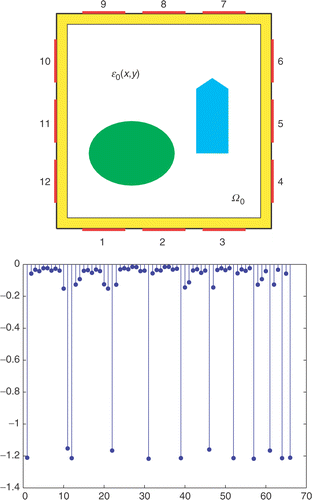
Electrode patches are placed around the periphery of the vessel wall ∂Ω for excitation voltage application and measurement collection. Suppose there are ℓ electrodes, labeled as Γ_i⊂∂Ω for i=1, 2,…,ℓ. In practice ℓ = 8, 12, 16, and 32 are common for various ECT sensor systems. There are gaps between neighboring electrodes. When the ith electrode serves as the single source electrode with normalized excitation voltage 1, the corresponding electric potential u_i(x,y) on Ω is governed by the following boundary value problem: (2) Here ν is the outward normal direction on ∂Ω, and δ_ik denotes the Kronecker delta: δ_ik=0 for k≠i and δ_ii=1. Then the mutual capacitance between electrodes i and j can be expressed as By Green's formula, this quantity can be expressed equivalently as an interior integral: (3) and these are much more convenient formulas of the capacitances for both analysis and computation. Note that each potential u_i=u_i(ε) depends on the permittivity distribution ε, and hence so do the capacitance data C_ij=C_ij(ε). Therefore (2.3) gives the full nonlinear model of the relation between the permittivity and the capacitance data. Because of the symmetry C_ij=C_ji and the relation , there are only ℓ₀=ℓ(ℓ−1)/2 independent capacitances. These and other properties of the capacitance data as a matrix [C_ij] are studied in 10. In the following, we arrange the ℓ₀ capacitance data as a vector (4) An example of a simulated data set (ℓ₀=66) is depicted in figure 1(b). Note that the number of measurements available is determined only by the number of electrodes placed on the sensor.

We remark that, in ECT, the entire sensor is usually enclosed by a screen to shield off other stray electromagnetic fields. Such an external screen can be incorporated into this model by proper modifications of the domain and boundary conditions, and our study here should still be applicable.

From (2.3), the first variation of C_ij due to variation ξ in ε₀ can be expressed explicitly as (5) where we have emphasized the dependence of each u_i on the reference permittivity ε, and used the fact that the variation ξ is zero on the vessel wall 8,9. These functionals are referred to as the sensitivity maps from permittivity to boundary capacitance data.

In fact, we can make the above variation statement more precise. Suppose the admissible class of permittivity distributions consists of those L^∞(Ω) functions ε that have the same value ε_wall in , and satisfy the bounds for some positive constants .

PROPOSITION 2.1

For any two admissible permittivity distributions ε and , there holds (6) Estimate (2.6) for the sensitivity maps provides a clearer indication to the validity of the linear approximation model (7) Roughly speaking, for this model to work well, it requires that the region where is not small has a small area.

The simplicity of the sensitivity maps (2.5) plays an important role in the design of reconstruction algorithms by level-set methods. The following property of these maps will also be relevant.

PROPOSITION 2.2

For an admissible ε(x,y), the corresponding sensitivity maps satisfy (8) for any B⊂Ω with |B|>0.

The proof of these two propositions are presented in the appendix.

3. Reconstruction algorithms by level-set method

In this section, we develop the iterative reconstruction algorithms that will provide simultaneous estimates for both the interfaces between phases and the permittivity values of the phases, from a given set of capacitance data . To this end, we seek a piecewise-constant function ε(x,y) that minimizes the following functional: (9) where C_ij is as given in (2.3), and J_reg(ε) is a regularization functional similar to the total variation of ε but in the specific form of piecewise-constant functions. The positive regularization constant α is usually chosen to be small. We set up iterative schemes for solving the Euler--Lagrange equations for the minimizer in the context of level-set formulation for piecewise-constant functions. We formulate the simpler two-phase problem first for a clearer introduction of the level-set methods, and then extend the framework to multi-phase situations.

3.1. Level-set formulation for two-phase flow

We first formulate the two-phase problem using level-set methods. In this case, each permittivity profile is described completely by the two permittivity values and the interface. Let φ(x,y) be a level-set function whose zero level curve φ(x,y)=0 is the interface between the two phases, and the two unknown permittivity values be τ₁ and τ₀. Specifically, we assume, for (x,y)∈Ω₀, It is more convenient to use the one-dimensional Heaviside function to express piecewise-constant functions, and the permittivity distribution ε in Ω can be written as (10) For the level-set function φ(x,y) in Ω₀, it is only the zero level set φ(x,y)=0 that is of interest, and the nonzero values of φ in Ω₀ are irrelevant.

We set the regularization functional to be the total variation of ε over the interior Ω₀: (11) which is the product of the jump between the regions and the arc length of the interface.

We seek our solution as the distribution ε that minimizes the functional (3.1) in terms of τ =(τ₁,τ₀) and φ =φ(x,y): (12) where C_ij(τ,φ) is as given by (2.3) using (3.2). We derive the associated Euler--Lagrange equations of J₁, and set up iterative schemes for finding the minimizer. Hence we suppose that a current estimate is represented by , and develop the equations for the new estimate ε in terms of (τ₁,τ₀,φ).

By a straightforward calculation using the sensitivity maps (2.5), we can obtain the Euler--Lagrange equations for J₁ with respect to (τ₁,τ₀): We use these equations to find approximate values for (τ₁,τ₀) when they are unknown. Thus, we use the available estimate to linearize the above system. Note that (13) where the quantities and W_ij are computed using the current estimate as In fact (3.5) is the linear model (2.7) in this situation. By further replacing (τ₁,τ₀,φ) with in the α-terms, we obtain the following linearized system for (τ₁,τ₀): (14) It can be seen that, if no regularization is present, this is in fact the normal equation for solving the linear system of ℓ₀ equations using the approximations of C_ij by (3.5). In the event when one of the τ's is known, say τ₀, we only need the first equation to obtain τ₁ (see (4.1) in the next section). Note that each diagonal in the coefficient matrix in (3.6) is exactly the quantity in (2.8) with B being the phase region, and hence is positive by Proposition 2.2 when the phase region has nonempty interior. This suggests that we may set up a Jacobi-type iteration to solve (3.6). In general, an additional regularization may be introduced to (3.6) by adding the term to the left of (3.6), with some small β > 0, so to prevent potential problems in solving (3.6) when the coefficient matrix becomes singular or ill-conditioned, such as when a phase region vanishes or becomes too small.

With (τ₁,τ₀) fixed, by a variational calculation, one can obtain the associated Euler--Lagrange equation for φ: in Ω₀, with boundary condition Here H′(s)=δ₀(s) denotes the one-dimensional Dirac delta function. The calculation for the arc-length part is standard (see e.g. 12,17,23), while that for the data-fitting term follows from the sensitivity maps (2.5). For effective numerical computation of the level-set function φ, the Heaviside function H and its derivative H′=δ₀ are often replaced by some smoothed approximations H_ϵ and , for example 3: (15) In this study, we only use δ_ϵ in place of H′=δ₀, and keep H in all its appearances. After a linearization, we embed the equation for φ in the evolution of φ =φ(t,x,y) (e.g. 23,3) according to (16) in (0,∞)×Ω₀, with boundary and initial conditions (17) Here t is an artificial time used as a parameter in the descent direction. We further apply one step in the implicit scheme for (3.8) to compute φ(x,y)=φ(Δt, x, y): (18) with the same boundary condition in (3.9).

Therefore, one iteration in our iterative schemes from to (τ,φ) consists of solving the linear system (3.6) for τ =(τ₁,τ₀) followed by solving the linear PDE (3.10) for φ.

Equation (3.8) evolves the level-set function φ on the entire domain Ω₀, although it is the zero level set of φ that is of interest. To prevent the degrading (e.g. flattening near the zero level set) of φ, it is a common practice to update this function while keeping the zero level set unchanged. This procedure is called re-initialization in the literature, referring to the update of φ to the signed distance function to the zero level set 12. An effective way of achieving such an update is to follow the evolution of d(t,x,y) to its steady state: (19) That is, we set the initial value of d to the level-set function φ to be updated, and obtain the update . Care should be taken in the numerical method of solving the hyperbolic equation (3.11) in order to keep the zero level set unchanged from φ to and to reach the steady state quickly, and we employ a monotone upwind scheme 13 that has been shown to be successful for this purpose. There are also various strategies on when to re-initialize (see e.g. 2,13), but we simply activate the re-initialization procedure after a fixed number of iterations, which is set to 200 in our numerical examples.

To determine if the iteration has reached a stationary state, we need to check if the zero level sets of φ and are close enough (see e.g. 23 for a criterion). Since here the permittivity values are part of the solution, we also need to check if the τ's have reached certain stable values/ranges.

The iterative algorithms for reconstructing the piecewise-constant permittivity distribution in terms of (τ₁,τ₀,φ) will be a special case of Algorithm 3.1 for the more general multi-phase problems.

We note that the regularization functional (3.3) we choose in this case is the same as the total variation of the permittivity distribution. Hence, when the two permittivity values τ₁ and τ₀ are known, the algorithms provide an effective way of including this a priori information in the reconstruction of the phase interface using TV regularization. On the other hand, if we absorb the scalar multiple |τ₁−τ₀| into the regularization parameter α, then this regularization is identical with the arc length regularization, and thus our method is the Mumford--Shah functional for piecewise-constant functions applied to ET problems. However, the situation is different in multi-phase problems, which is to be discussed next.

3.2. General multi-phase formulation

With K level-set functions (φ₁, φ₂, … , φ_K), we can represent up to 2^K distinct regions of the form (see 19,2), and each may be used to represent a phase. For an m-phase flow, we need level-set functions, even if there are redundant regions. Since we will be finding the permittivity values for the phases too, we assign one value for each region, and let the algorithms decide if some of the values are approximately the same. In the event that we do know exactly how many phases there are in the flow, we can combine some of the regions to represent one phase so to eliminate the redundancy in regions. In general, there may be as many as 2^K algebraic equations in a system like (3.6) for the 2^K permittivity values, and K partial differential equations like (3.8) for the level-set functions (φ₁,φ₂,…,φ_K). Instead of formulating the problem in general terms, we illustrate the idea with the simple but representative case of K = 2.

Suppose the 4 possible permittivity values are , in association with the 4 regions given by the two level-set functions through the representation of the interior permittivity distribution ε₀(x,y) in Ω₀ as follows. (20) Then we can write with We set the regularization functional for this case to be (21) Since we see that this regularization is between the TV regularization and the arc length regularization . Like TV regularization, the weights |g_k| provide some control on the permittivity differences across the interfaces; on the other hand, the expression of (3.13) is much simpler than the total variation of ε₀ in this specific setting of piecewise-constant functions, which enables us to apply the variational level-set method for the Euler--Lagrange equations below.

The objective function (3.1) is then dependent on and φ =(φ₁,φ₂), expressed as (22) where C_ij(τ,φ) is given by (2.3) for ε given by (2.1) and (3.12). Here we use a single regularization parameter α for both level-set terms, with local jump-relevant adjustments from |g₁| and |g₂|. If necessary, we can use two different regularization parameters α₁ and α₂ for the two terms separately.

We will derive the associated Euler--Lagrange equations of J₂ with respect to τ and φ, and set up iterative schemes for solving them, using the current estimate represented by and . We describe next how the new estimate ε is obtained by finding and φ =(φ₁,φ₂).

For τ =(τ₁₁,τ₁₀,τ₀₁,τ₀₀), we can obtain the associated Euler--Lagrange equations by using the sensitivity maps (2.5) and a simple calculation on the regularization term: (23) where the vector p consists of the 4 phase indicators: and stands for the 4×2 Jacobian matrix of (g₁, g₂) with respect to (τ₁₁,τ₁₀,τ₀₁,τ₀₀). To linearize (3.15), as in (3.5), we approximate the capacitance C_ij(τ,φ) by (24) for 1≤i<j≤ℓ, where the quantities are defined similarly as in the two-phase case; e.g., These quantities are dependent on and , but are independent of τ. Again, (3.16) is the specific form of the linear model (2.7) in this case. By arranging the entries according to (2.4), we write these ℓ₀ expressions of (3.16) in vector form as (25) Note that each of the vectors is nonzero by Proposition 2.2 provided that the corresponding phase region has nonempty interior. Substituting these approximations and using the current estimate and for p and the α-terms in (3.15), we obtain a linear system for the new estimate τ =(τ₁₁,τ₁₀,τ₀₁,τ₀₀): (26) where the ℓ₀×4 matrix , and the 4-vector r is explicitly given by with (k≠k′). Again we see that (3.18) is the normal equation for the ℓ₀ approximate equations with additional small terms due to regularization. If only some of the τ values are unknown, we will use only the corresponding equations from (3.18); see e.g. (4.3) in the next section for a case of two unknown τ's. From Proposition 2.2, each diagonal entry of A^T A is positive if the corresponding phase is present. In order to avoid potential problems of A^T A being singular or ill-conditioned when solving (3.18), such as in the situation where a phase region vanishes or becomes very small, we may add a regularization term of to the left of (3.18).

As for (φ₁,φ₂), by a similar variational calculation as for the two-phase case, we have in Ω₀, with boundary conditions for k, k′=1, 2 with k≠k′. Here denotes the derivative of with respect to h_k=H(φ_k), and in this (K = 2) case . After linearization, we embed (φ₁,φ₂) in the evolution of (27) in (0,∞)×Ω₀, with boundary and initial conditions (28) (k, k′=1, 2 with k≠k′). Here . Again we employ one step in the implicit scheme for (3.19) to obtain φ_k(x,y)=φ_k(Δt, x, y) in (29) with the same boundary condition in (3.20). We see from here that |g₁| and |g₂|, the weights in the regularization functional for the arc lengths, can be viewed as either adjustments to the regularization parameter on each level-set, or adjustments to the time step Δt in solving the level-set evolution equations by (3.21).

It is clear that the above derivation is readily applicable to the general case of K > 2 interface functions with 2^K possible phase regions, provided that the permittivity distributions are expressed similarly as in (3.12) using the 2^K permittivity values and phase regions. One convenient notation system for the expression is the use of binary indexes for these 2^K values and the corresponding phase regions (see e.g. 2). Once the notation system is chosen, the g_k's and thus the regularization functional can be computed accordingly (g_k is independent of φ_k), and the equations for both the permittivity values and level-set functions can be set up in the same way as we have described above for the case of K = 2.

In summary, our iterative algorithms for reconstructing multi-phase permittivity profiles can be described as follows.

Algorithm 3.1 (Multi-phase permittivity reconstruction)

1.	ν = 0: Choose initial (τ(0),φ(0)). For example, and the signed distance function of a simple contour.
2.	Use (τ(ν),φ(ν)) to construct the permittivity profile by (3.2) or (3.12), and solve the associated forward problem (i.e. ui's from (2.2)) to obtain data , as well as the quantities and w.
3.	Solve the linear system (3.6) or (3.18) to obtain τ =τ(ν +1). If only some of them are unknown, only the relevant equations in (3.6) or (3.18) are used. If all are known, this step is skipped.
4.	Set , and solve for from (3.10) or (3.21) for each k.
5.	When necessary, re-initialize to the signed distance function to its zero level set.
6.	Check if the solution is stationary. If not, set ν =ν +1 and repeat.

4. Numerical implementation and examples

In this section, we describe our discretization methods, and present numerical examples of implementing the reconstruction algorithms proposed in the previous section.

In our numerical experiments, we choose the scaled domain Ω as the unit square (0,1)×(0,1). We assume that the sidewall has a thickness of t₀=0.04, and the ℓ = 12 electrode patches are of the same width of 0.20, evenly placed on ∂Ω with 3 on each side and a gap of 0.08 between neighboring patches on the same side, as depicted in the left of figure 1. Therefore, there are ℓ₀=66 independent capacitance measurements to be used for reconstructing the permittivity profile, no matter what size of discretization we introduce on Ω.

4.1. Discretization by finite element/difference methods

On Ω, we set up uniform rectangular grid with Δx=Δy=1/n for a given natural number n. We use the two sets of grid points for discretization: grid points of for the elliptic problems of (2.2), and centers of the grid rectangles for the permittivity distributions and the level-set functions.

For the elliptic boundary value problems (2.2), we apply the finite element method where the basis functions are the tensor products of the one-dimensional linear elements: Thus the potentials u(x, y) are represented by their nodal values of u_ij=u(x_i,y_j) on the grid points as . In these calculations, the permittivity distribution ε(x,y) in (2.2) is assumed constant on each grid rectangle; therefore we choose accordingly the discrete representation of ε by its values at the centers of the rectangles . The gradient product ∇u·∇v for two potentials u and v is needed for the calculation of the sensitivity maps and other quantities, and we approximate this on each grid rectangle by its corresponding average value; that is, Note that, by the finite element approximation, the two components of a potential gradient are linear functions of either y or x, respectively, in each rectangle R_ij.

To be consistent with the discretization of the permittivity distributions, we represent a level-set function φ(x,y) by its values . For the level-set equations (3.10) or (3.21) as well as their re-initializations (3.11), we use finite difference approximations. For the divergence operator in (3.10) or (3.21), we use where and the forward and backward difference operators are defined as usual: As for the re-initialization equation (3.11), we use the following upwind scheme 13, from to d_ij with time-step ω: where and the sign function is approximated by It is known that this scheme is stable if , and we carry out a fixed number of steps for the solution to be close enough to the steady state. Since we do not activate this re-initialization process often, it does not add much to the overall computational load of the reconstruction algorithms.

4.2. Numerical examples

In our numerical examples below, we set Δx=Δy=1/50 (n = 50). The Dirac delta function δ₀ is approximated by δ_ϵ in (3.7) with ϵ =1.5Δx, while no approximation for the Heaviside function H is used. We activate the re-initialization (3.11) for the level-set functions once after every 200 iterations. The 66 capacitance data to be used are generated by adding random noise to the simulated data: where c(ε^(true)) is the data set simulated using the true distribution ε^(true), rand represents a 66-vector of random numbers from the uniform distribution on [−1,1], and η is the relative noise level. For each example, we run the algorithms on simulated data with noise from several different draws from the MATLAB random number generator, and select a typical result to present.

When the τ values are to be found simultaneously with the interfaces, we set the following ensuring constraints on them: These are imposed by projection after each of their updates in the iteration process, i.e. after Step 3 in Algorithm 3.1. In most of the cases we have tested, these constraints are not active, and in some cases they are active only for a few iterates when the level-set functions experience large changes. In a few examples, we need to impose stricter bounds in order for the iteration to continue, and these are clearly situations when the associated level-set functions undergo dramatic changes. Such constraints can be considered as extra a priori knowledge for the unknown material flow, and they are not stringent at all in practice since there are often obvious bounds available for certain permittivity values.

Reconstruction results largely depend on the relative noise level η and choice of the regularization parameter α. There are certain types of profiles that are more tolerant to larger noise levels than others. Instead of using different noise levels in different examples, we set η =0.05% for all the two-phase examples and η =0.02% for the multi-phase examples, for a better comparison between various permittivity profiles. As for the regularization parameter α, we choose one among a few convenient choices we tested, and it is by no means the “optimal” in any sense. Generally speaking, larger α works better for larger scale and smoother profiles without much detail, while smaller α is needed to capture some details in the profile in smaller scale and with less smoothness.

Initial guesses for the interfaces may also affect the performance of the reconstruction algorithms. In the two-phase examples, the algorithms seem to be convergent from many different initial profiles we have tested, with the only difference being in the number of iterations. Hence, we set the same initial guess in all the two-phase example as the signed distance function of a small circle in the center, for a fair comparison among all examples. On the other hand, for the multi-phase examples when the permittivity values are fixed, we do need good initial guesses for most cases in order to produce reasonable results. We set the initial guesses for the two unknown phases as the signed distance functions of two small circles near the center, and they are relatively close to their corresponding true interfaces. However, if the permittivity values are computed along with the shape evolution process, this has not been a problem in all the examples we have tested. For comparison purposes, we use the above-mentioned choice of the initial guesses for all of our multi-phase examples, with or without fixed permittivity values. Finally, initial guesses for any unknown τ's do not affect the performance of the iteration algorithms. These experiments seem to suggest a practical strategy in dealing with the dependence on good initial guesses: even in the event that the permittivity values are a priori known, we should allow the permittivity values to vary according to the algorithms, and only to insert their given values near the end of the iteration to improve the shape estimates.

We set the time step size in (3.10) to Δt=5Δx for two-phase examples, and Δt=2.5Δx in (3.21) for multi-phase examples. Larger Δt often causes instability in the iteration process, while smaller Δt would require more iterations.

It is possible (and perhaps more desirable) to establish some stopping criteria to automatically check on the steady-state status of the iterations (see e.g. 23). In our experiments we terminate the iteration after some fixed number of iterations or when some convergence is observed in the data errors , in the computed τ values, and in the changes of the zero level set. In these specific examples to be presented next, after we determine to terminate, we make certain that there are no significant changes in the reconstruction results even if more iterations are carried out.

4.2.1. Two-phase examples

In the case of two phases, we set τ₀=1 throughout, representing the gas/air as the background phase. We test two methods: one for reconstructing only the interface function φ with known permittivity value τ₁=2, and the other for solving both φ and τ₁ simultaneously. In the first case, we need not solve equations in (3.6), and we only solve for φ by the iteration (3.10). When τ₁ is unknown, we modify the equation for τ₁ in (3.6) to (30) In all these examples, we have also tested the case when both τ₁ and τ₀ are to be computed by (3.6), and we have found that the recovered τ₀ is almost exact while the reconstruction results for both τ₁ and φ are very similar.

We choose a variety of interface profiles to test the algorithms. Instead of selecting profiles that are easy to recover by our algorithms (such as relatively large regions without much details), we design our test profiles to explore how well our algorithms can perform against some challenging features, or how ill-posed the ECT problem is with respect to these profiles.

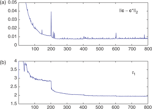
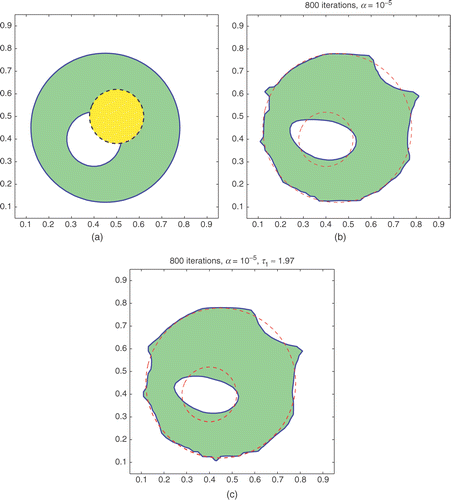
In Example A1, the non-gas phase region is relatively large but with an inner opening. The objective here is to test the recovery of both outer and inner boundaries simultaneously. As shown in figure 2, from the initial circle, the algorithms find the interior opening by the automatic deformation of the level-set function, and recover the outer boundary reasonably well at the same time. A selected sample of the shape evolution sequence (when τ₁=2 is fixed) is presented in figure 3. When τ₁ is computed during the course of the iteration, the data errors and the computed τ₁ are shown in figure 4, and it can be seen that the iteration process is very much stable and convergent. Moreover, this is one of these cases where the algorithms are more tolerant to noise, and our tests showed that with a higher η (e.g. 0.5%) the reconstruction results were still quite satisfactory.

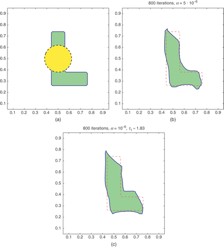
Figure 2. Example A1. (a) The true profile (solid) and the initial guess (dashed). (b) Reconstructed result for φ with τ₁ = 2 fixed. (c) Reconstructed result for both φ and τ₁ computed.

Figure 3. Shape evolution for Example A1 when τ₁=2 is fixed.

Figure 4. (a) Data errors and (b) computed τ₁ over the iterations, for Example A1 in figure 2(c).

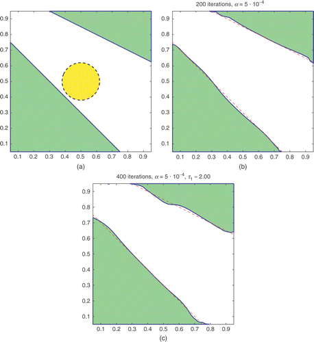
In Example A2 we test the case of straight-line interfaces that meet the sidewall in an angle (figure 5a). When starting the initial profile in the small circle in the center, we observe that the level-set function φ undergoes dramatic changes: the region {φ >0} starts to spread, then breaks up into some smaller regions, which finally merge to form the two separated regions, with the help of a re-initialization step. It is more so in the case of computed τ₁ (a sample of the shape evolution sequence is presented in figure 6), and we do need to impose a stricter lower bound for τ₁ when it is not known: 1.1≤τ₁≤10. It is observed that this stricter constraint is active only during the first few iterations when the regions starting to spread and break up, but it is crucial to have this bound in place so to prevent the iteration be trapped in some local minimum of the optimization problem. This case also can tolerate higher levels of noise in the data.

Figure 5. Example A2. (a) The true profile (solid) and the initial guess (dashed). (b) Reconstructed result for φ with τ₁ = 2 fixed, without re-initialization. (c) Reconstructed result for both φ and τ₁ computed, where a stricter lower bound of 1.1 for τ₁ is active only in the first few iterates.

Figure 6. Shape evolution for Example A2 where τ₁ is computed throughout the process.

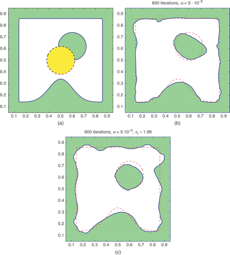
Example A3 in figure 7(a) is designed to test the deformation of the interface into a large surrounding region with the breakout of a smaller interior region. As can be seen, the algorithms work very well in reconstructing both the interfaces and the permittivity value, with a good amount of details of the interfaces recovered. Again, in the case of computing both τ₁ and φ, we need to set the lower bound of 1.1 for τ₁, due to large changes in φ.

Figure 7. Example A3. (a) The true profile (solid) and the initial guess (dashed). (b) Reconstructed result for φ with τ₁ = 2 fixed. (c) Reconstructed result for both φ and τ₁ computed, where a stricter lower bound of 1.1 for τ₁ is active only in the first few iterates.

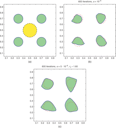
In Example A4, the non-gas phase region consists of 4 smaller circles, as shown in figure 8(a). The difficulty in this case is the smaller size of the regions. When the permittivity value τ₁ is known, the reconstruction of the interfaces is quite accurate. When τ₁ needs to be computed, the algorithms seem to settle with slightly larger regions and a lower value of τ₁. This profile seems to be more sensitive to noise level in data.

Figure 8. Example A4. (a) The true profile (solid) and the initial guess (dashed). (b) Reconstructed result for φ with τ₁ = 2 fixed. (c) Reconstructed result for both φ and τ₁ computed.

In Example A5, the true region is an L-shape in the center (figure 9a). It is challenging to recover the overall shape that has a narrow width and a 270○-corner in the inside. Our algorithms seem to be able to reconstruct the interface well, especially when τ₁ is known. If τ₁ is also computed by the algorithms, then the algorithms settle for a more spread region with a lower value of τ₁. This profile is also sensitive to noise.

Figure 9. Example A5. (a) The true profile (solid) and the initial guess (dashed). (b) Reconstructed result for φ with τ₁ = 2 fixed. (c) Reconstructed result for both φ and τ₁ computed.

4.2.2. Three-phase examples

In the following we present some examples using Algorithm 3.1 for three-phase permittivity profile reconstruction. In (3.12), we assume that τ₀₀=τ₁₁=1 and these two phase regions are combined to represent the gas/air phase. Thus the permittivity distribution can be expressed equivalently as (31) Again we test two methods: one for reconstructing only the two interfaces φ₁ and φ₂ by assuming the exact values of τ₁₀ and τ₀₁, and the other for computing both the interfaces φ₁, φ₂ and the permittivity values τ₁₀, τ₀₁ for the two non-gas phases. With τ₁₀ and τ₀₁ given, we only need to advance the two level-set functions by using (3.21); that is, Step 3 in Algorithm 3.1 is skipped. If τ₁₀ and τ₀₁ are unknown, we modify the linear system (3.18) into the following form so as to have the equations for these two unknowns only: (32) Together with (3.21) for the level-set functions, we simultaneously reconstruct the unknown interfaces and the two permittivity values.

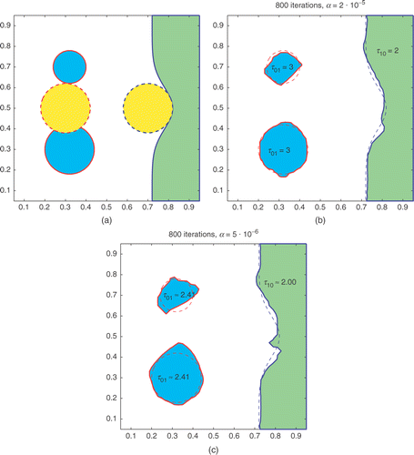
In all examples, we set the initial guesses as the two signed distance functions of the two small circles, the right for the τ₁₀-phase and the left for the τ₀₁-phase.

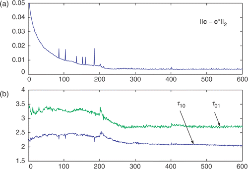
In Example B1, the two true interfaces are a circle for the τ₁₀-phase and a square for the τ₀₁-phase; see figure 10(a). Reconstructed interfaces by both methods are very accurate (see figure 10b, c), while the computed value for higher permittivity τ₀₁ is less accurate than the computed value of the lower τ₁₀. In figure 11, we plot the data errors as well as the computed τ₁₀ and τ₀₁ versus the iteration number, which show that the iteration process is stable and convergent. For this example, we have also tested the dependence on initial guesses in the case of fixed (τ₁₀,τ₀₁)=(2,3). When the initial guesses for the two phases are switched (level-set functions remain the same), each initial phase region is now farther away from its true phase region and closer to the other true phase region, and the iteration seems incapable of driving each phase region toward its true location; instead, each phase region is drawn toward the location of the other true phase region but with a larger/smaller shape. However, this problem does not occur if we allow (τ₁₀,τ₀₁) to evolve with the shapes according to the algorithms.

Figure 10. Example B1. (a) The true profiles (solid) and the initial guesses (dashed) for φ₁ (right) and φ₂ (left). (b) Reconstructed result for (φ₁,φ₂) with (τ₁₀,τ₀₁) = (2, 3) fixed. (c) Reconstructed result for (φ₁,φ₂) and (τ₁₀,τ₀₁) computed.

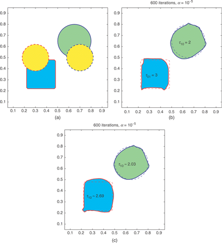
Figure 11. (a) Data errors and (b) computed (τ₁₀,τ₀₁) over the iterations, for Example 1 in figure 10(c).

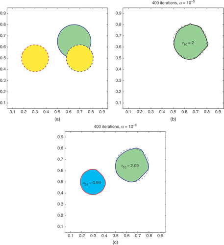
In the next two examples, we test the algorithms when used on data from two-phase distributions. In Example B2 (figure 12), the non-gas phase region is only the circular region with τ₁₀=2 (i.e. τ₀₁=τ₁₁=τ₀₀=1 in (4.2)). Without this knowledge, we apply the three-phase reconstruction algorithms to the data, with the same initial guesses for the two non-gas phases as in Example B1. When τ₀₁ is fixed at 3, the interface for that phase (the zero level-set of φ₂) automatically disappears, at the same time as the interface for τ₁₀=2 phase being recovered accurately; see figure 12(b). On the other hand, when both the interfaces and τ-values are being computed, the zero level-set of φ₂ does not vanish; instead, the value for the corresponding τ₁₀ is adjusted to nearly the background value of 1, indicating the absence of this phase in a different way (figure 12c). Therefore, in this example, both methods produce accurate reconstruction results.

Figure 12. Example B2. (a) The true profile (solid) and the initial guesses (dashed) for φ₁ (right) and φ₂ (left). The true phase of τ₀₁=3 is absent. (b) Reconstructed result for (φ₁,φ₂) with (τ₁₀,τ₀₁) = (2, 3) fixed. Note that the phase τ₀₁ automatically disappears. (c) Reconstructed result for (φ₁,φ₂) and (τ₁₀,τ₀₁). The computed τ₀₁ is nearly the same as the background phase of τ₁₁=τ₀₀=1, and thus the interface by φ₂ is unnecessary.

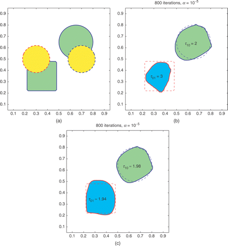
The true distribution in Example B3 is also two-phase, but the non-gas phase region (τ₁₀=2) now consists of two separated parts: the circle and the square (see figure 13a). With τ₀₁ and τ₁₀ fixed at 3 and 2, the algorithms would not eliminate the τ₀₁-phase, but settle for a smaller region (figure 13b). On the other hand, when τ₀₁ is allowed to evolve with the iteration process, the algorithm is able to find its correct value and thus recover the two-phase profile accurately.

Figure 13. Example B3. (a) The true profiles (solid) and the initial guesses (dashed) for φ₁ (right) and φ₂ (left). The true phase of τ₀₁=3 is absent. (b) Reconstructed result for (φ₁,φ₂) with (τ₁₀,τ₀₁) = (2, 3) fixed. Note that the phase τ₀₁ does not vanish in the reconstruction, and thus the true profiles are not correctly recovered. (c) Reconstructed result for (φ₁,φ₂) and (τ₁₀,τ₀₁). The computed τ₀₁ and τ₁₀ are close enough to indicate the absence of the third phase; the true profiles are recovered correctly.

In Example B4, the two interfaces are very different: the τ₁₀-phase has a relatively larger region near the domain boundary, and the τ₀₁-phase consists of two smaller interior circles. To reach these profiles from the same initial profiles, it requires different deformation paths (splitting vs. spreading). As can be seen in figure 14, our algorithms successfully provide the needed evolution for the level-set functions φ₁ and φ₂ to yield accurate reconstruction results for the interfaces. In the case of fixed (τ₁₀,τ₀₁), we show a sample of the shape evolution sequence in figure 15. For the case when (τ₁₀,τ₀₁) are computed by the algorithms, because of the larger changes in φ₁, we need to impose a stricter lower bound of 1.1 for τ₁₀ and τ₀₁. Although this constraint is only active in the first few iterates, it helps to keep the deformations of the interfaces along the right paths.

Figure 14. Example B4. (a) The true profiles (solid) and the initial guesses (dashed) for φ₁ (right) and φ₂ (left). (b) Reconstructed result for (φ₁,φ₂) with (τ₁₀,τ₀₁) = (2, 3) fixed. (c) Reconstructed result for (φ₁,φ₂) and (τ₁₀,τ₀₁) computed, where a stricter lower bound of 1.1 for both τ₁₀ and τ₀₁ is active only for the first few iterates.

Figure 15. Shape evolution for Example B4 when (τ₁₀,τ₀₁)=(2,3) are fixed.

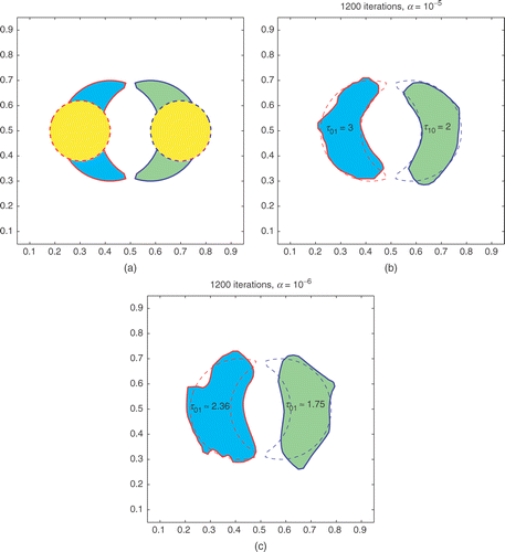
In Example B5, the two phases have crescent-shape interfaces (see figure 16a), which have similar concave/narrow-width feature as the L-shape in Example A5. With known exact values of τ₁₀ and τ₀₁, the recovered interfaces are quite accurate. When τ₁₀ and τ₀₁ are to be computed, the reconstructed regions are more spread-out and with lower computed values of τ₁₀ and τ₀₁, similar to the situations in Examples A4 and A5.

Figure 16. Example B5. (a) The true profiles (solid) and the initial guesses (dashed) for φ₁ (right) and φ₂ (left). (b) Reconstructed result for (φ₁,φ₂) with (τ₁₀,τ₀₁) = (2, 3) fixed. (c) Reconstructed result for (φ₁,φ₂) and (τ₁₀,τ₀₁) computed.

5. Conclusions

We have developed numerical algorithms for reconstructing multi-phase permittivity of material flow from capacitance data in electrical capacitance tomography. Using the level-set representation for the piecewise-constant permittivity profiles, we set up iterative algorithms that give both interface and permittivity estimates simultaneously. The regularization functional we have introduced is most suitable for this type of problem, since it inherits the natural form of arc-lengths for the application of level-set methods, and retains the desirable regularization effect of total variation. The interface estimates are obtained by the interface evolution based on a variational level-set method, and the permittivity estimates are found by solving linear systems along the iteration process. The simultaneous reconstruction of interfaces and permittivity values is convenient and effective, and provides flexibility and independence on initial interface selections, even in the event when the permittivity values are a priori known. Our numerical experiments have shown that the algorithms are capable of providing accurate reconstruction results of multi-phase permittivity distributions in both the interface locations and unknown permittivity values.

Appendix

In the following we complete the proof for the properties of the sensitivity maps stated in Propositions 2.1 and 2.2.

Proof of Proposition 2.1

Let u_i=u_i(ε) be the H¹ weak solution to (2.2) with respect to ε. That is, u_i∈H¹(Ω) with u_i=δ_ik on Γ_k satisfies (33) for all φ∈H¹(Ω). Then, for the solutions u_i(ε) and corresponding to ε and respectively, we have (34) where in the last step we have used the test functions of and in the equations for u_i(ε) and u_j(ε), respectively. On the other hand, from the equations for u_i(ε) and with , we have which leads to By applying the above estimate in the last term of (A2), we can obtain (2.6).▪

Proof of Proposition 2.2

If otherwise, the sum in (2.8) is zero, then each term in the sum is zero: We proceed to show a contradiction. Since in Ω (10), . Therefore, the above implies that That is, u_i ≡ c_i (constant) in B. The maximum principle for u_i asserts that 0≤u_i≤1 on Ω (10), hence we have 0≤c_i≤1 for each 1≤i≤ℓ and .

Suppose B₀ is an open disk such that . Denote . From (A1), since ∇u_i=0 in B₀, we have (35) for all ψ∈H¹(Ω′), and in particular, with ψ =u_i, (36) Let v be the H¹-weak solution to the following boundary value problem in Ω′: (37) Therefore, (38) for all ψ∈H¹(Ω′), and there holds the maximum principle 0≤v≤1 on . If we use ψ =v in (A3), we have (39) By setting ψ =u_i and ψ =v in (A6), we obtain respectively (40) Because the c_i's are nonnegative and , there is at least one nonzero c_i, say c₁ > 0. From (A3) and (A6), we have for all ψ∈H¹(Ω′). Set ψ =u₁−v as a test function in the above to obtain: Hence, a contradiction, since c₁ > 0 and, as the unique solution to (A5), v cannot be a constant in Ω′.

Therefore, we conclude that (2.8) is true.▪

References

- Beck, MS, Dyakowski, T, and Williams, RA, 1998. Process tomography—the state of the art, Measurement and Control 20 (1998), pp. 163–177.
- Chan, T, and Tai, X-C, 2003. Level set and total variation regularization for elliptic inverse problems with discontinuous coefficients., Journal of Computational Physics 193 (2003), pp. 40–66.
- Chan, T, and Vese, L, 2001. Active contour without edges, IEEE Transactions on Image Processing 10 (2001), pp. 266–277.
- Cheney, M, Isaacson, D, and Newell, JC, 1999. Electrical impedance tomography, SIAM Review 41 (1999), pp. 85–101.
- Chung, E, Chan, T, and Tai, XC, 2005. Electrical impedance tomography using level set representation and total variation regularization, Journal of Computational Physics 205 (2005), pp. 357–372.
- Dobson, D, 1997. "Inverse Problems in Imaging and Nondestructive Testing". In: Engl, H, Louis, AK, and Rundell, W, eds. Recovery of blocky images in electrical impedence tomography. Wien: Springer-Verlag; 1997. pp. 43–64.
- Dyakowski, T, Jeanmeure, LFC, and Jaworski, AJ, 2000. Applications of electrical tomography for gas–solids and liquid–solids flows—a review, Powder Technology 112 (2000), pp. 174–192.
- Fang, W, 2004. A nonlinear image reconstruction algorithm for electrical capacitance tomography, Measurement and Science Technology 15 (2004), pp. 2124–2132.
- Fang, W, 2006. Reconstruction of permittivity profile from boundary capacitance data, Applied Mathematics and Computation 177 (2006), pp. 179–188.
- Fang, W, and Cumberbatch, E, 2005. Matrix properties of data from electrical capacitance tomography, Journal of Engineering Mathematics 51 (2005), pp. 127–146.
- Ito, K, Kunisch, K, and Li, Z, 2001. Level-set function approach to an inverse interface problem, Inverse Problems 17 (2001), pp. 1225–1242.
- Osher, S, and Fedkiw, R, 2003. Level Set Methods and Dynamic Implicit Surfaces. Springer-Verlag: New York; 2003.
- Peng, D, Merriman, B, Osher, S, Zhao, H, and Kang, M, 1999. A PDE-based fast local level set method, Journal of Computational Physics 155 (1999), pp. 410–438.
- Reinecke, N, and Mewes, D, 1996. Recent developments and industrial research applications of capacitance tomography, Measurement and Science Technology 7 (1996), pp. 325–337.
- Rondi, L, and Santosa, F, 2001. Enhanced electrical impedance tomography via the Mumford--Shah functional, ESAIM Control, Optimisation and Calculus of Variations 6 (2001), pp. 517–538.
- Rudin, LI, Osher, S, and Fatemi, E, 1992. Nonlinear total variation based noise removal algorithms, Physica D 60 (1992), pp. 259–268.
- Sethian, JA, 1996. Level Set Methods and Fast Marching Methods. Cambridge University Press: Cambridge; 1996.
- Soleimani, M, Lionheart, W, and Dorn, O, 2006. Level set reconstruction of conductivity and permittivity from boundary electrical measurements using experimental data, Inverse Problems in Science and Engineering 14 (2006), pp. 193–210.
- Vese, L, and Chan, T, 2002. A multiphase level set framework for image segmentation using the Mumford amd Shah model, International Journal of Computer Vision 50 (2002), pp. 271–293.
- Yang, WQ, and Peng, L, 2003. Image reconstruction algorithms for electrical capacitance tomography, Measurement and Science Technology 14 (2003), pp. R1–13.
- Yang, WQ, Stott, AL, and Beck, MS, 1995. Development of capacitance tomographic imaging systems for oil pipeline measurements, Review of Scientific Instruments 66 (1995), pp. 4326–4332.
- York, TA, 2001. Status of electrical tomography in industrial applications, Journal of Electronic Imaging 10 (2001), pp. 608–619.
- Zhao, H, Chan, T, Merriman, B, and Osher, S, 1996. A variational level set approach to multiphase motion, Journal of Computational Physics 127 (1996), pp. 179–195.