Numerical differentiation and its applications

Abstract

Differentiation is one of the most important concepts in calculus, which has been used almost everywhere in many fields of mathematics and applied mathematics. It is natural that numerical differentiation should be an important technique for the engineers. However, since it is ill-posed in Hadamard's sense, which means that any small error in the measurements will be enlarged, it is very difficult for the engineers to use this technique. In this article, we propose a new simple numerical method to reconstruct the original function and its derivatives from scattered input data and show that our method is effective and can be realized easily.

Keywords:

• Numerical differentiation
• Ill-posedness
• Tikhonov regularization
• Error analysis

1. Introduction

The derivative is one of the most important concepts in calculus. It is used in all fields of mathematics and applied mathematics. Moreover, this concept has also been accepted by most researchers in other fields and engineers.

It is well known that derivatives are used to describe how a function changes. In many practical problems, the understanding of most physical phenomena involves the determination of derivatives of the original function. However, numerical differentiation techniques are not often used by the engineers. The reason is that the numerical differentiation problem is an ill-posed problem in the sense of Hadamard, which means that any small error in the measurement may cause huge errors in the numerical approximation (refer 1–3). This difficulty made the engineers find other ways to avoid the numerical differentiation as sometimes simple problems can become very complicated. It is desirable that, if some new stable algorithms for numerical differentiation can be proposed, the numerical differentiation technique will become a powerful tool for the engineers.

We just mention possible applications of the numerical differentiation technique, for example, the determination of discontinuous points in image processing 4; the solution of Abel integral equation 5; and some inverse problems arising from mathematical and physical equations 2, etc.

There are several ways to treat the numerical differentiation problem. The most common and simplest way, which is used by the engineers, is finite difference. One of the disadvantages of this method is that, in the case that the data contains errors, even if we have many data, we cannot use all data. In other words, the size of the grid cannot be too small. This seems difficult for the engineers because they have to know more about the algorithm according to the original problem. This disadvantage is due to the ill-posedness of the numerical differentiation problem. To overcome this difficulty, several methods have been proposed, for example, Tikhonov regularization method 3, mollification method 6, etc.

In this article, we will apply Tikhonov's regularization technique to reconstruct higher-order derivatives from scattered data. The feature point of our method is that we can overcome the most difficult step in Tihkonov's regularization, by giving a simple strategy of choosing the regularization parameter which also implies the same convergence rate as the usual choice strategy. For another related work on higher-order numerical differentiation, we can refer to 7.

It should be remarked that Tikhonov's regularization technique has been shown to be quite effective for treating many ill-posed problems 1,6,8 and it has been used to treat numerical differentiation problems by Hanke and Scherzer 2 and Wang et al. 9,10. However, most results are about first-order derivatives.

The article is organized as follows: In section 2, we give the formulation of the problem. In section 3, the main theoretical results are presented and proved. We give the algorithm in section 4. Some applications are given in section 5.

2. Formulation of the problem

Suppose that y=y(x) is a function defined on [0,1] and x_n=1} is a uniform grid of [0,1] where n is a natural number. Let δ > 0 be the level of noise in the data. Let .

We consider the following numerical differentiation problem: given some noisy samples of the function values y(x_i) which satisfies we want to construct a function f_*(x) such that the derivatives of f_*(x) are approximations of the derivatives of function y(x).

Without losing the generality, we may assume that

Recall the following notations for the Sobolev spaces: whose norms are defined by

Here the superscript (l) denotes the l-th order derivative with respect to x.

Let k > 1 be an integer and n > k. We denote

We define the following cost functional (1) where the function and α is a regularization parameter.

It can be shown that there exists a unique minimizer for the functional Φ, i.e. (2) for any function .

We will show that the minimizer f_* is one of the solutions of the numerical differentiation problem.

3. Main theoretical results

For the functional Φ, we have:

THEOREM 3.1

There exists one unique function such that for any functions .

Proof

We will prove this theorem in several steps:

Step 1

Construction of the minimizer f_*.

First we assume that there exists a minimizer . Define a function where g(x)∈H^k satisfies g(0)=g(1)=0. Since f_* is the minimizer of the functional Φ(f), then we have F^′(0)=0. (3)

Hence, we have

Since g∈H^k can be an arbitrary function, it can be verified that 12 and f_* satisfies the following boundary conditions: (4) and (5) We then have where δ(x) is the Dirac delta function. Hence, we obtain (6)

In other words, when x≠x_j, f_* satisfies: (7) and, when x = x_j, f_* satisfies: (8)

It can now be concluded that is a distribution and .

For any g(x)∈H^k which satisfies: (9) we have

Therefore, we have

Let ε→0. We can obtain that and finally we have (10) for

The solution of (3.5) is then given as: (11) where the 2kn parameters , k=1,2,…, 2k, j=0,1,…,n-1, are determined by solving the following 2kn linear equations:

Next, we will prove that these linear equations with respect the unknown constants , k=1,2,…, 2k, j=0,1,…,n-1 are uniquely solvable. For proving this, we only need to show that the homogenous equations have only the trivial solution.

If we choose , j=0,1,2,…,n, then by the same step we did before, the linear equations we obtained are just the homogenous equations. On the other hand, from the definition of the functional Φ, we know that is the unique function that minimizes Φ. This means that the homogenous equations have only the trivial solution. Hence, there exists a unique solution for the equations.

Step 2

The function f_* is the unique minimizer of the functional Φ.

For any functions , we denote . It is obvious that g(0)=g(1)=0 and (12)

Here, the difference of the norms is given by

Hence, we have

It means that the function f_* is a minimizer of the functional Φ(f).

If there is another function f₁ such that , then from Step 1 we have and thus is a polynomial of degree k − 1. Since , n > k, the polynomial has more than k − 1 roots which is a contradiction. Therefore, we have which means that the minimizer f_* is unique.

The proof is completed.▪

Remark 3.2

From the proof of Theorem 3.1, we know that is a piecewise polynomial of degree 2k-1 which can be determined by 2kn parameters.

One important thing is how to choose the regularization parameter α in the functional Φ so that the minimizer can be one possible solution of the numerical differentiation problem. The strategy we use in this article is a very simple one, i.e. we take α = δ². This is motivated by the results in 11, in which it is shown that the conditional stability implies the convergence rate of the Tikhonov regularization solution under this simple strategy of choosing the regularization parameter.

We have the following convergence rate results.

THEOREM 3.3

Suppose that f_* is the minimizer of the functional Φ and α = δ². If y∈H^k(0,1), then we have (13) where 0≤j≤k-1, K_1j, and K_2j are constants depending on j which can be seen in the proof.

Remark 3.4

The assumption y∈H^k(0,1) is the same as the source condition which is used in Tikhonov regularization 8. Actually if we denote , then y∈H^k(0,1) is equivalent to .

Before proving Theorem 3.3, we first prove several lemmas.

LEMMA 3.5

Let , , and f is a function that has m-th order derivative in (a, b). There exists a constant K which depends on ε₀, p, and b-a such that for every ε, 0≤j < m, we have (14)

This is a standard result in Sobolev spaces. The proof can be found in, for example, 12.

LEMMA 3.6

Let , h be the mesh size defined in section 2, and let δ denote the level of noise. We have (15)

Proof

From the definitions of Φ and f_*, we have (16)

Then, it can be obtained that (17)

By simple calculation, we have and

Therefore, we obtain (18)

The proof is completed.▪

Next we will give the proof of Theorem 3.3.

Proof of Theorem 3.3

We denote .

First we prove: (19) where K₁, K₂ are two constants independent of h and δ.

Taking and f = e in Lemma 3.5, we can obtain

Without losing the generality, we assume that .

We take . Then we have

Since we obtain

From Lemma 3.6, we have (20)

Next we will show that (3.17) can be obtained from (3.18). We consider two cases

Case 1 . Then it is obvious that (3.17) is true.

Case 2 . Then we take .

We rewrite (3.18) as (21)

It can be obtained that

Therefore, we have (22)

The inequality (3.17) is proved.

By a similar method, we can prove that, for any 0≤j < k, it holds that

We will not give the detailed proof here.

This completes the proof of Theorem 3.3.▪

In the following, we will consider what happens for the regularized solution if the exact solution does not have enough regularity. Actually, it will be seen later that this result can be used to identify the nondifferentable points of the function y 9.

THEOREM 3.7

Take α = δ². Suppose that f_* is the minimizer of the functional Φ. If , then we have

We will not give the proof here. The reader can find the proof in the case k = 2 in 9. For general k, the proof is similar.

Remark 3.8

Without any change, our method works for the general interval [a,b]

Remark 3.9

The two dimensional numerical differentiation problems have been treated by the same techniques. The readers can find the results in. 13 and 14.

4. Algorithm

We consider the simple case k = 3. The other cases can be treated in a similar way.

Since f_* is a piecewise polynomial of degree five, we assume that where there are 6 n constants a_i, b_i, c_i, d_i, e_i, f_i, i=0,…, n-1.

From our construction, we have

By the boundary conditions, we can obtain (23)

We denote it as (24)

We denote it as (25)

We denote it as where y_i, i=1,…,n-1, are given data

Finally, we get the following matrix equation: (26)

By solving (4.4) and using the above matrix relations, we can get the coefficient vectors a_j, b_j, c_j, d_j, e_j, and f_j for j=1, 2,…, n-1.

Then , and .

The constant c₀ can be obtained from the equality . From , we can get f₀. By , we can obtain b₀.

The details can be found in 15.

5. Application

In this section, we will give three applications of our numerical differentiation method.

5.1. The inverse problems of identifying coefficients in a boundary value problem

We consider the following nonlinear ill-posed problems, i.e., the identification of the coefficient c in the two-point boundary value problem from the solution u.

It is a typical nonlinear ill-posed problem which has been treated by Tikhonov regularization by many researchers (8,16 etc). It is obvious that this problem can be simply regarded as a numerical differentiation problem. By the technique we proposed in a previous section, we can treat this problem very easily. We can get c directly from

The example we take here is that and .

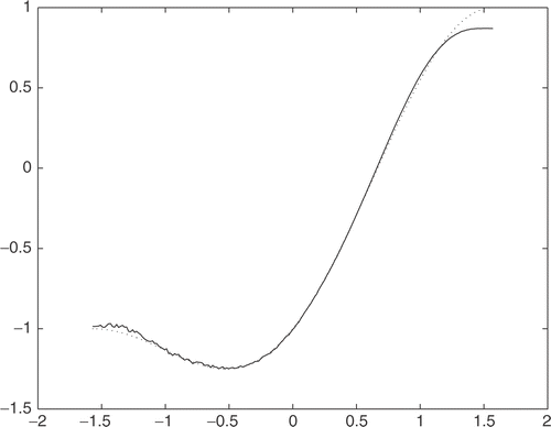
We choose k = 3 and use the algorithm in section 4. The numerical results are shown below.

In our computation we let n = 200 and δ = 0.005. In this case . Noisy data are generated by adding some random errors to the exact values. The error is controlled by δ. The numerical result is displayed in figure 1 where the dotted line represents u′ and the solid line represents . It can be observed that the values of u′ and are perfectly matched. The error estimate of the first order derivative is acceptable.

Figure 1. Comparison of the first derivatives between the exact u′ (dotted line) and its approximation (solid line).

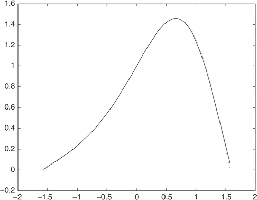
In figure 2, the dotted line represents u′′ and the solid line represents . We can also observe that u′′ and matches well.

Figure 2. Comparison of the second derivatives between the exact u′′ (dotted line) and its approximation (solid line).

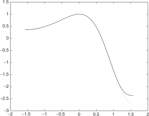
In figure 3, the dotted line represents c and the solid line represents . We can also observe that c and matches well too.

Figure 3. Comparison of the exact c (dotted line) and its approximation (solid line).

5.2. Determination of the interface in computerized tomography

This example is to show how to apply the results of Theorem 3.7 to a very simple, but interesting problem in Computerized Tomography (CT) 17. Here we just give a brief description. Some details can be found in 9.

We assume that the attenuation coefficient of an object with respect to an X-ray at x is f(x). We scan the cross-section by an X-ray beam L of unit intensity. The intensity past the object is

We denote

The main problem in CT is to recover the function f from g.

If one wants to reconstruct the function f completely, the inversion formula should be used. However, in many cases, it will be enough if one can reconstruct the interface of the different mediums. It should be remarked here that the nondifferentiable points of g is related directly with the discontinuous points of f. In the following, it is shown that, by our numerical differentiation method, the discontinuous points of f (x) can be determined easily. These discontinuous points represent the interface of different mediums. This can be used to reconstruct the shape of the object.

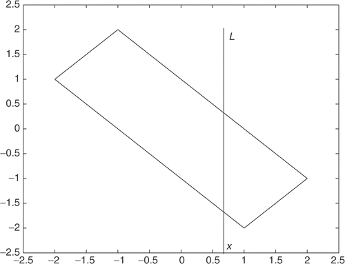
We consider a simple case of an object whose cross section is a rectangle which we denote by D. The attenuation coefficient is 0 outside the object and 1 inside the object, i.e., (27)

See figure 4.

Figure 4. Picture of D and L.

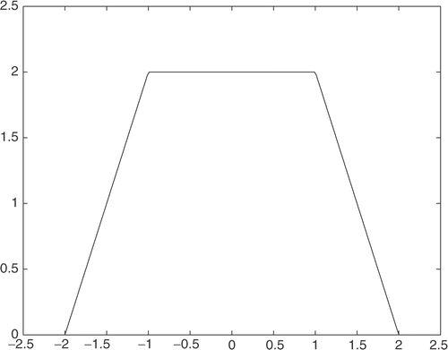
Function g(x) can be calculated directly (28)

See figure 5. It is easy to see that there are four discontinuous points.

Figure 5. Picture of g.

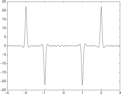
By our method, we choose 201 points as x_i, i=0,1,2,…,200, and reconstruct g′(x) from (here ε_i is a random error whose value is less than 0.001.) The second-order derivative is shown in figure 6. From figure 6, we can find that the values of are large near four points: -2,-1,1,2, and are almost 0 at other points. By this fact, we can easily find the nondifferentiable points.

Figure 6. Picture of .

5.3. Reconstruction of the local volatility by Dupire formula

The Black–Scholes equation is (29) where V is the option premium which is determined by several factors including the underlying asset price S, current time t, the maturity date T, the exercise price K, the risk-free interest r, the dividend yield on the asset q and the local volatility σ. The volatility measures the riskiness of the underlying asset.

The inverse problem of option pricing (IPOP) is to deduce the local volatility surface σ(S,t). In other words, we would like to determine the pair of functions V(S,t;K,T) and σ(S,t) by using the current market prices (30) where is the underlying asset price at the current time .

If option prices are known for all possible strikes K and expirations T then the local volatility function can be theoretically found directly from the following formula: (31)

This simple formula was found by Dupire in 18. However, even this formula, which only contains the derivatives of the stock price, is so simple it has not been used by the researchers for a long time. The reason is the ill-posedness of the numerical differentiation. Recently, Ye and Yi used the numerical differentiation technique proposed in this paper and got some nice results 19.

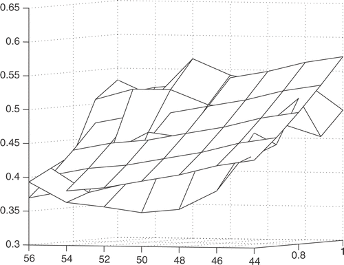
In the Dupire formula, the values of stock price function V are given at some discrete points, (K_j, T_j) , j=1,2,…, N. The constants r, q are given.

Therefore this is a numerical differentiation problem. We calculate the numerical derivative along T direction and K direction separately. Figure 7 presents one of the numerical results. The reader can find the details in 19.

Figure 7. Picture of local volatility (numerical result and exact solution).

6. Conclusion

In this article, we proposed a simple effective numerical method for the numerical differentiation problem. The simplest strategy of choosing the regularization parameter works very well and it makes our algorithm be realized very easily. Some applications are presented.

The two-dimensional numerical differentiation problems have been treated by the same techniques. The readers can find the results in 13 and 14.

Acknowledgments

The authors would like to thank the anonymous referees for their comments and suggestions which are very important for the revision of this article. This research is partly supported by NSF of China (No. 10271032, No. 10431030). The first named author is also partly supported by the Shuguang Project and E-Institute of Shanghai Municipal Education Commission (N.E03004).

References

- Groetsch, CW, 1984. "The theory of Tikhonov regularization for Fredholm equations of the first kind.". In: Research Notes in Mathematics. Vol. 105 . Boston, Mass.–London: Advanced Publishing Program; 1984, Pitman.
- Hanke, M, and Scherzer, O, 2001. Inverse problems light: numerical differentiation., Inverse problems light: numerical differentiation. 108 (6) (2001), pp. 512–521.
- Tikhonov, AN, and Arsenin, VY, 1977. Solutions of Ill-posed Problems. Washington: Winston & Sons; 1977.
- Deans, SR, 1983. Radon Transform and its Applications. New York: A Wiley-Interscience Publication, John Wiley & Sons Inc.; 1983.
- Gorenflo, R, and Vessella, S, 1991. "Abel Integral Equations, Analysis and Applications". In: Lecture Notes in Mathematics. Vol. 1461. Berlin: Springer-Verlag; 1991.
- Murio, DA, 1993. The Mollification Method and the Numerical Solution of Ill-posed Problems. New York: A Wiley-Interscience Publication, John Wiley & Sons Inc.; 1993.
- Anderssen, RS, and Hegland, M, 1999. For numerical differentiation, dimensionality can be a blessing!, For numerical differentiation, dimensionality can be a blessing! 68 (227) (1999), pp. 1121–1141.
- Engl, HW, Hanke, M, and Neubauer, A, 1996. Regularization of Inverse Problems. Dordrecht: Kluwer Academic Publishers Group; 1996.
- Wang, YB, Jia, X.Z, and Cheng, J, A numerical differentiation method and its application to reconstruction of discontinuity., Inverse Problems 18, pp. 1461–1476.
- Jia, XZ, Wang, YB, and Cheng, J, 2003. The numerical differentiation of scattered data and it's error estimate., The numerical differentiation of scattered data and it's error estimate. 25 (2003), pp. 81–90.
- Cheng, J, and Yamamoto, M, 2000. One new strategy for a priori choice of regularizing parameters in Tikhonov's regularization., One new strategy for a priori choice of regularizing parameters in Tikhonov's regularization. 16 (2000), pp. L31–L38.
- Adams, RA, "Sobolev spaces". In: Pure and Applied Mathematics. Vol. 65. New York-London: Academic Press.
- Wei, T, Hon, YC, and Wang, YB, 2005. Reconstruction of numerical derivatives from scattered noisy data., Reconstruction of numerical derivatives from scattered noisy data. 21 (2) (2005), pp. 657–672.
- Wang, YB, and Wei, T, 2005. Numerical differentiation for two-dimensional scattered data., Numerical differentiation for two-dimensional scattered data. 312 (1) (2005), pp. 121–137.
- Lu, S, and Wang, YB, 2004. The numerical differentiation of first and second order with Tikhonov regularization., The numerical differentiation of first and second order with Tikhonov regularization. 26 (2004), pp. 62–74.
- Jin, QN, 2000. Error estimate of some Newton-type methods for solving nonlinear inverse problems in Hilbert scales., Error estimate of some Newton-type methods for solving nonlinear inverse problems in Hilbert scales. 16 (2000), pp. 187–197.
- Natterer, F, 1986. Teubner, BG, ed. The Mathematics of Computerized Tomography. Stuttgart: John Wiley & Sons, Ltd., Chichester; 1986.
- Dupire, B, 1994. Pricing with a smile., Pricing with a smile. 7 (1994), pp. 18–20.
- Yin, B, and Ye, Y, 2006. Recovering the local volatility in Black-Scholes model by numerical differentiation., Recovering the local volatility in Black-Scholes model by numerical differentiation. 16 (2006), pp. 681–692.