Simultaneous estimation of temperature-dependent thermal conductivity and heat capacity based on modified genetic algorithm

Abstract

An inverse heat conduction analysis is presented to simultaneously estimate the temperature-dependent thermal conductivity and heat capacity based on a modified elitist genetic algorithm (MEGA). In this study, MEGA is used to minimize a least squares objective function containing estimated and simulated (filtered) temperatures. The estimated temperatures are obtained from the direct numerical solution (finite differences method, or FDM) of the finite one-dimensional conductive model by using an estimate for the unknown temperature-dependent thermophysical properties (TDTPs). The accuracy of the MEGA is assessed by comparing the estimated and the preselected TDTPs. The results of the MEGA are used as the starting point for a locally convergent optimization algorithm, i.e., the Levenberg–Marquardt (L–M) method. It is shown in this work that hybridization of the MEGA with the L–M method can lead to accurate estimates. From the results, it is found that the RMS error between estimated and simulated temperatures is very small irrespective of whether measurement errors are included or excluded. In addition to estimation of the TDTPs, sensitivity analysis is performed to investigate the effects of heating duration. Also, it is found that the results of the MEGA are highly satisfactory with only single-sensor measurements on the heated surface.

Keywords:

• Inverse heat conduction
• Parameter estimation
• Genetic algorithm
• Temperature-dependent thermophysical properties

1. Introduction

Estimation of the temperature-dependent thermophysical properties (TDTPs) is an imperative problem because of its significant influence on heat transfer and temperature distribution 1. For example, the temperature rise and heat conducted through the surface for a mild steel (AISI 1020) rubbing pair, sliding at 6 m s⁻¹ and with 30 N nominal load, predicted by the TDTPs solution is about 30% higher than that predicted using a constant thermal properties assumption 2.

Inverse problems of estimating TDTPs have been generally solved by using the conjugate gradient method with adjoint problem for parameter estimation or a common gradient-based method such as Gaussian linearization and modified Box–Kanemasu methods 3. In case there is no prior information about the functional form of unknown TDTPs or in the case of simultaneously estimating correlated parameters, such techniques are very difficult to apply because of their sensitivity to measurement errors.

Huang and Ozisik 4 applied a direct integration approach to estimate linear TDTPs. Their algorithm is not very sensitive to the choice of initial guesses, sensor location, and experiment times, but needs curve-fitted measurements. Chen et al. 5 used the hybrid application of the Laplace transform technique and the finite difference method (FDM) to estimate the temperature-dependent thermal conductivity using measured nodal temperatures inside the material. Five thermocouples must be inserted into the tested material in order to obtain a more accurate estimation of TDTPs in this approach. Huang et al. 6, 7 applied the conjugate gradient method to estimate the temperature-dependent thermal conductivity k(T) and heat capacity c(T). At least two thermocouples were used for estimating k(T) 7.

Two different versions of the Levenberg–Marquardt (L–M) method and four different versions of the conjugate gradient method were compared for the identification of the three thermal conductivity components of an orthotropic cube 8. The use of the L–M method resulted in the smallest CPU times and RMS error of the estimated parameters.

Most of the works found in the literature are based on gradient methods, whereas some use different approximation and direct integral methods such as the Laplace transform and Duhamel theorem 9–11. Such methods do not take into account measurement errors and are limited to linear cases. Genetic algorithm (GA) is a robust, nongradient algorithm that belongs to the field of evolutionary algorithms. Garcia developed an excellent GA code to optimize the experiment design for estimation of TDTPs of composite materials 3.

Davis 12 has shown that hybridization of GA and local gradient-based methods, rather than using any of them in isolation, can lead to better performance. The use of such hybrid GA would exploit the advantages of both GA and local methods, and seems a promising strategy for solving ill-posed inverse heat transfer problems with interesting computation cost.

2. Direct problem

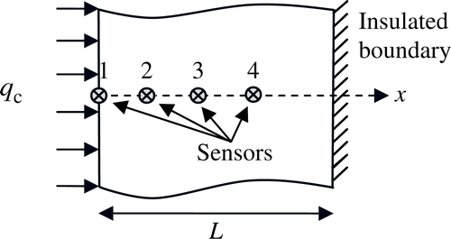
Consider a one-dimensional homogeneous slab as shown in figure 1 with thickness L and initial temperature T_init. The thermal conductivity k(T) and specific heat capacity c(T) are unknown. The boundary surface at x = 0 is subjected to a prescribed constant heat flux q_c, and the boundary surface at x = L is kept insulated. Employing a thin stainless steel foil as a heater guarantees that the applied heat flux enters the specimen, and this is beneficial because we can neglect the thermal effects of the heater. The governing differential equation of this problem can be expressed as: (1) and boundary conditions are in the following forms: (2) (3) where t_h is heating duration, and the initial condition is: (4) For the direct heat conduction problem, the temperature distribution in the slab as a function of space and time can be numerically (FDM) determined 13 provided that all TDTPs of the slab are given. Conversely, unknown TDTPs can be estimated only when additional information on temperature in the slab is given. In order to simulate the experiment, the temperature histories at some sensor locations are usually measured in the slab. We use the temperature histories taken from the heated surface and denoted them by , i = 1, … , I, where I denotes the number of the time readings.

Figure 1. One-dimensional conductive model.

3. Measurement simulation

The measured temperature data, , used in the present inverse analysis can be determined from the exact temperature solution of the direct heat conduction problem with the given TDTPs, T_exact. Owing to experimental uncertainty, contains the measurement error. Thus, T_exact should be modified by Gaussian additive noise in order to simulate experimental measurements. With respect to the eight statistical assumptions in reference [14, Chapter 1, p. 10], can be expressed as: (5) where σ is the standard deviation of the temperature measurements and ϵ is a random variable ranging from −2.576 to 2.576 for normally distributed errors with zero mean and 99% confidence bounds. The product of ϵσ represents the temperature measurement error.

4. Inverse analysis

Inverse parameter estimation methods are based on the minimization of an objective function containing both estimated and measured temperatures 14, 15. Ordinary least squares (OLS) estimator is by far the most frequently used method for the estimation of TDTPs as no prior knowledge is needed 15. OLS estimator was considered in this research. The associated objective function, the least squares error, S, is expressed by 16: (6) where β is the estimated parameter vector containing the unknown TDTPs; is the ith observation from the mth sensor; M and I are the number of sensors and observations, respectively. T_im(β) is the calculated temperature from the mathematical model governing the heat transfer phenomena with respect to the estimated parameter vector.

In using equation (6), the thermal properties are found by minimizing the sum of squared differences between the measured and calculated data. The minimization of equation (6) could conceivably be performed by any optimization technique. However, parameter estimation has generally been performed with only a few methods. The use of one method over another is often specific to a certain field of study. The approach investigated in the present work involves the use of a robust nongradient method, namely the GA method, in the minimization procedure. The motivation for using GAs was to circumvent difficulties of nonconvergence in cases when the parameters are correlated or nearly so.

5. Genetic algorithm

GAs were developed by Holland 17. The common feature of these algorithms is to simulate the search process of natural evolution and take advantage of the Darwinian survival-of-the-fittest principle. In short, evolutionary algorithms start with an arbitrarily initialized population of coded individuals with size n_s, in which a population P consists of individuals c_i with i = 1, … , n_s: (7) The population evolves toward increasingly better regions of the search space by means of both random and probabilistic methods (or deterministic methods in some algorithms). An individual is a possible solution of an optimization problem with the objective function S(β), which is a scalar-valued function of an n-dimensional vector β. The vector β consists of n unknown parameters β_j, with j = 1, … , n, which represent a point in real space Rⁿ. The variable β_j is called a gene. Thus, an individual c_i consists of n genes: (8) The goodness of each individual is evaluated by a fitness function that is defined from the objective function of the optimization problem. To define a fitness function for minimization problems such as equation (6), it is necessary to change the objective function, because GA works according to the principle of the maximization of the fitness function, and so the fitness function of equation (6) is defined as: (9) The square root function is included to moderate the selection pressure of the GA, and 0.01 is added arbitrarily to limit the maximum of the fitness function and avoid the infinity.

The basic operators used in GAs consist of selection (the selection of parents for breeding), crossover (the exchange of parental genes to create children) and mutation (the changing of individual genes) 18. The most popular and easiest mechanism to select parents is the roulette wheel selection (RWS), where each individual in the current population has a roulette wheel slot sized in proportion to its fitness. An arithmetic crossover 19 is applied to each pair of the mating pool with a crossover probability, P_c. A mutation operator modifies gene values of individuals according to a mutation probability, P_m. In addition, following the Darwinian theory, an elitism operator (the protection of best individuals), e.g., generational replacement with probability P_r is used, in which parents are replaced with children, while the n_s × (1 − P_r) best parents are kept 17. The most widely used stopping criterion, e.g., number of generation n_g, is used in this work.

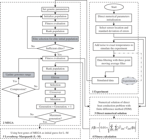
Goldberg developed the basic elitist genetic algorithm (BEGA). In this work, BEGA is modified with some additional operators such as an elite initial population and a domain compression operator. The modified elitist genetic algorithm (MEGA) started by a successive random search for elite individuals in which only the first-ranked individual of each initial population is kept for an elite initial population. The procedure used by the MEGA to generate the elite initial population is presented in figure 2. A compression factor r_c is then applied in some generations to reduce the parameters’ search space as follow: (10) (11) where U_i and L_i are upper and lower bounds of the ith gene of individuals, respectively. And c_best,i is the ith gene of the first-ranked individual in the generation in which the domain compression operator is applied.

Figure 2. Flowchart of the proposed method.

There are many advantages of applying GAs to estimation problems. GAs are easily programmed. Their major strength is that they are derivative-free calculations and, as shown in this work, they do not need any initial guesses. Another strength of GAs is their capability to hybridize with other techniques such as gradient-based methods. Although the GA is a powerful technique for estimation, it does have certain weaknesses in comparison to gradient-based methods. Design of robust GAs is highly application-specific and their performance is difficult to predict. Another significant drawback is the high CPU cost.

A mathematical function called f6 12, 20 was optimized to illustrate the performance of the MEGA. The expression of this function is: (12)

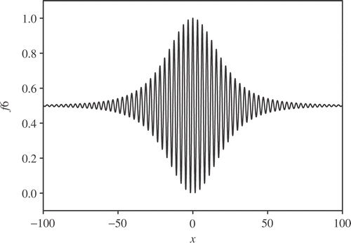
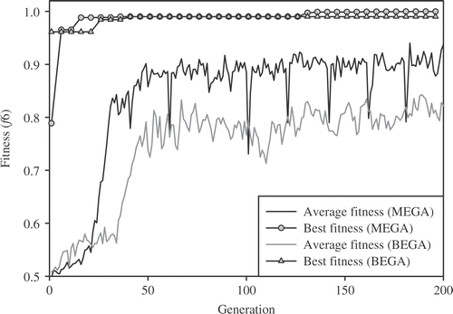
Figure 3 illustrates the distribution of this function with y being held constant at its optimal point while x ranges from −100 to 100. The goal is to optimize f6, e.g., to find values of x and y that produce the greatest possible value for f6. This function has some interesting features such as a single global optimum, which is f6(x = 0, y = 0) = 1, strong oscillations, and a tiny fraction of the total area for the global regions. Figure 4 shows a typical increase of both the fitness (function f6) of the best individual and the average fitness of the population obtained from the BEGA and MEGA. As illustrated in figure 4, MEGA is more effective than BEGA to find the global optimum of the test function. Also, the average fitness of MEGA is greater than that of BEGA.

Figure 3. Function f6 vs. x with y set to 0.

Figure 4. Average and the best fitness evolution of function f6.

6. Methodology

A flowchart of the proposed method for TDTPs estimation is shown in figure 2. A simulated experiment was performed with adding Gaussian white noise to the exact solution of the direct conductive model. To simulate the experiment, the preselected TDTPs are assumed for two cases of dependency as: (13) (14) (15) (16) Dimensionless time and heating duration are defined as: (17) where α is the average thermal diffusivity of the sample and t_f is the total measurement time. Constant heat flux q_c = 120 kW m⁻² is applied at the left boundary; measurement interval is chosen as 1.25 s. A total of 1600 simulated measurements containing additive, uncorrelated, and normally distributed errors with zero mean and constant standard deviation of σ = 0.01T_max were assumed available for the estimation procedure, where T_max is the maximum of the exact temperature in the simulated experiment.

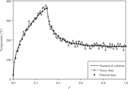
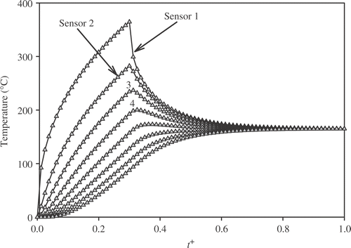
Simulated measurements of temperature at the heated surface and some internal locations are presented in figure 5 for heating duration . Actual measured data could be used for the inverse analysis as illustrated in figure 2. A three-point moving-average filter is applied to reduce measurement errors. Filtered temperatures at the heated surface are compared with noisy measurements in figure 6. After completion of data filtering, these measurements are used in MEGA to estimate the unknown TDTPs. After the MEGA optimization process, the best genes of the last generation are used as an initial guess for the L–M algorithm.

Figure 5. Simulated measurements of temperature at the heated surface and some internal locations for .

Figure 6. Filtered temperatures with σ = 0.01T_max at the heated surface for .

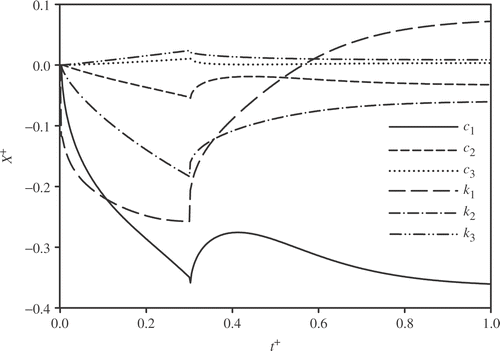
Sensitivity coefficients provide information that may be used to understand and design experiments 21, 22. In general, the scaled dimensionless sensitivity coefficients are desired to be large for each parameter and uncorrelated (linearly independent) for different parameters. 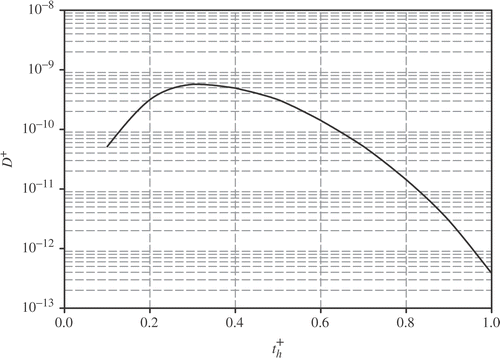A sense of the magnitude of the sensitivity coefficients is gained through normalizing the sensitivity coefficients and is performed by multiplication of parameters for all scaled sensitivity coefficients as follows: (18) By using a separate finite difference code, these coefficients are computed for the current experimental design (case of parabolic TDTPs) and are shown in figure 7. A criterion is needed to identify an optimum design 23. Dimensionless D-optimality 15 is selected because of its relation to the volume of the confidence region for the estimated parameters and expressed as: (19) This criterion maximizes the determinant of the information matrix where | | denotes the determinant, superscript T the transpose symbol, and F⁺ dimensionless Fisher information matrix. The maximum temperature constraint provides consistency when comparing experiments that may have different temperature ranges 22, 24, and so the effects of heating duration on the dimensionless D-optimality criterion are investigated and shown in figure 8. In order to attain a constant maximum temperature rise for different heating duration times, the magnitude of the heat flux must be chosen appropriately. It is found that using a dimensionless heating duration of 0.3 maximizes the D-optimality criterion.

Figure 7. Scaled dimensionless sensitivity coefficients of parabolic TDTPs for .

Figure 8. Effect of the heating duration on the dimensionless D-optimality criterion for estimating parabolic TDTPs.

7. Results and discussion

Genetic parameters could affect the convergence and performance of the MEGA. There are unfortunately few heuristics to guide a user in the selection of appropriate operators and genetic parameter settings for a particular problem. What can be grasped from the literature is that good GA performance requires the choice of a moderate population size, a high crossover probability, and a low mutation probability 3. So, genetic parameters in the current research are chosen as: n_s = 100; n_g = 1000; P_c = 0.99; P_m = 0.05; P_r = 0.9; r_c = 0.9. The valid ranges for the unknown parameters are specified to begin the MEGA search, e.g., c ∈ (0–2000) and k ∈ (0–500). The ranges of the second and third parameters in equations (13–16) are obtained from the functional form of the unknown TDTPs considering the above valid ranges.

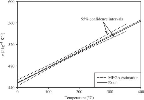
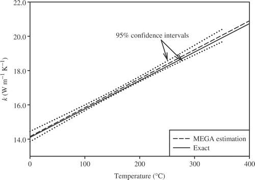
The inverse estimation of TDTPs is first performed by assuming exact measurements for the linear dependency case. Then, analysis is repeated for the noisy measurements with σ = 0.01T_max for both linear and parabolic TDTPs. As randomness plays an important role in each run of the MEGA (two runs with different random seeds will generally produce different output), five different runs and their mean with 95% confidence intervals are presented in tables 1 and 2 for both exact and noisy measurements.

Table 1. Estimation of linear TDTPs using MEGA and L–M method with genetic parameters: n_s = 100, n_g = 1000, P_c = 0.99, P_m = 0.05, P_r = 0.9, and r_c = 0.9 for σ = 0 and σ = 0.01T_max

Run			c1	c2	k1	k2	RMS error
σ = 0	MEGA	1	448.17	0.295	14.12	0.0165	0.033
		2	448.55	0.299	14.14	0.0164	0.059
		3	446.60	0.285	14.03	0.0169	0.109
		4	448.78	0.306	14.16	0.0163	0.082
		5	447.21	0.280	14.09	0.0168	0.097
		Mean	447.86 ± 1.15	0.293 ± 0.013	14.11 ± 0.06	0.0166 ± 0.0005	0.076 ± 0.038
	L–M		448.00	0.291	14.10	0.0166	1e−8
σ = 0.01Tmax	MEGA	1	450.41	0.275	14.28	0.0160	2.10
		2	446.87	0.311	13.88	0.0173	2.08
		3	449.86	0.273	14.19	0.0169	2.11
		4	448.63	0.285	13.93	0.0175	2.09
		5	446.25	0.314	14.25	0.0165	2.10
		Mean	448.40 ± 2.25	0.292 ± 0.024	14.11 ± 0.232	0.0168 ± 0.0008	2.10 ± 0.01
	L–M		447.22	0.304	14.14	0.0167	2.08
	L–M*		447.69	0.296	14.12	0.0166	1.85
*Estimation with filtered data.

Table 2. Estimation of parabolic TDTPs using MEGA and L–M method with genetic parameters: n_s = 100, n_g = 1000, P_c = 0.99, P_m = 0.05, P_r = 0.9, and r_c = 0.9 for σ = 0.01T_max

Run			c1	c2	c3	k1	k2	k3	RMS error
σ = 0.01Tmax	MEGA	1	446.92	0.5237	−4.9e−4	13.70	0.0197	−2.31e−5	2.83
		2	445.64	0.5121	−5.2e−4	13.97	0.0209	−1.92e−5	2.91
		3	449.78	0.5386	−4.3e−4	14.28	0.0205	−1.84e−5	2.78
		4	443.21	0.5069	−5.3e−4	13.56	0.0208	−2.03e−5	2.85
		5	445.11	0.5425	−4.5e−4	14.13	0.0196	−2.12e−5	2.94
		Mean	446.10 ± 3.03	0.5248 ± 0.020	−4.8e−4 ± 5e−5	13.93 ± 0.37	0.0203 ± 0.001	−2.03e−5 ± 7e−7	2.86  ± 0.08
	L–M		446.42	0.5296	−5.0e−4	13.94	0.0205	−2.05e−5	2.51
	L–M*		447.35	0.5387	−5.2e−4	13.98	0.0204	−2.12e−5	2.18
*Estimation with filtered data.

In this work, it is assumed that the form of the estimated TDTPs is priori unknown as in most real-world engineering applications. One may choose different forms of the unknown estimated TDTPs and calculate the RMS error between simulated and estimated temperatures to find minimum RMS error. As presented in table 3, when simulation is based on the linear form, the linear form of the unknown estimated TDTPs yields a minimum RMS error. Similarly, for the parabolic case, use of the parabolic form for the unknown estimated TDTPs gives a minimum RMS error.

Table 3. Estimation of linear and parabolic TDTPs with respect to the different functional forms of the estimates

Simulation	Estimation	c1	c2	c3	k1	k2	k3	RMS error
Linear TDTPs	Constant	566.13	–	–	17.69	–	–	6.37
	Linear	447.69	0.296	–	14.12	0.0166	–	1.85
	Parabolic	444.67	0.311	−7.2e−5	13.91	0.0187	−4.6e−6	4.37
Parabolic TDTPs	Constant	548.35	–	–	17.23	–	–	5.23
	Linear	451.89	0.247	–	14.31	0.0147	–	3.39
	Parabolic	447.35	0.5387	−5.2e−4	13.98	0.0204	−2.12e−5	2.18

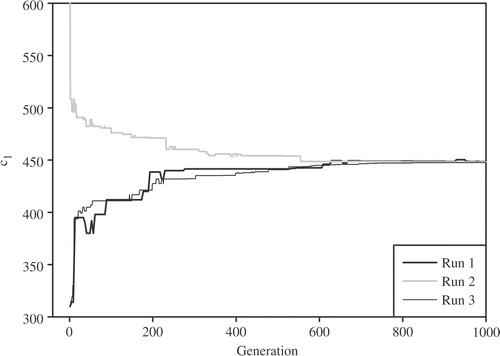
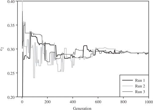
The best and average fitness of the MEGA for the parabolic TDTPs estimation are presented in figure 9. As illustrated in this figure, three different runs of the MEGA converge at the generation number of 1000. Estimated heat capacity parameters for linear TDTPs are presented in figures 10 and 11.

Figure 9. Average and the best fitness evolutions of function f(β) from the MEGA for parabolic TDTPs with σ = 0.01T_max.

Figure 10. Estimated heat capacity parameter (c₁) from the MEGA for linear TDTPs with σ = 0.01T_max.

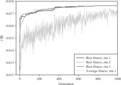
Figure 11. Estimated heat capacity parameter (c₂) from the MEGA for the linear TDTPs with σ = 0.01T_max.

The estimates obtained from the MEGA are then used as an initial guess for the L–M method, which results in accuracy and fast convergence. A damping parameter of 0.001 is chosen for the L–M method, and the damping matrix is taken from diagonal elements of the Fisher information matrix. Estimates are also obtained with filtered data for linear, and parabolic TDTPs are tabulated in tables 1 and 2. From the results, it is found that using filtered data could improve the accuracy of the estimates. It is clear that L–M method provides a more accurate estimation when appropriate initial estimates are chosen from the MEGA. CPU times for each separate run of MEGA on a Pentium IV processor at 2800 MHz and 1 GB of RAM are about 160 and 170 s for linear and parabolic cases, respectively.

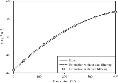
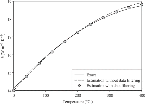
The results that are obtained from the exact measurements (σ = 0) in table 1 show an excellent agreement between estimates and preselected TDTPs. As we can see, the RMS error between simulated and estimated temperatures is very small (equal to 1e−8). The estimated specific heat capacity and thermal conductivity with σ = 0.01T_max are compared with the preselected linear TDTPs in figures 12 and 13 and the parabolic TDTPs in figures 14 and 15, respectively.

Figure 12. Estimated heat capacity for the linear TDTPs with σ = 0.01T_max.

Figure 13. Estimated thermal conductivity for the linear TDTPs with σ = 0.01T_max.

Figure 14. Estimated heat capacity for the parabolic TDTPs with σ = 0.01T_max.

Figure 15. Estimated thermal conductivity for the parabolic TDTPs with σ = 0.01T_max.

95% confidence intervals of estimates are also shown in figures 12 and 13. Small confidence intervals clarify the accuracy of the MEGA. As noted before and shown in figures 14 and 15, using filtered data could improve the accuracy of the estimates.

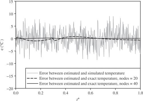
Residual distribution is a proper way to investigate the accuracy of the proposed method, and is shown in figure 16 for two numbers of nodes. A small signature was found in the residual distribution at the end of the heating duration when the number of nodes is small, e.g., 20. As illustrated in figure 16, by using smaller spatial and time step intervals in the direct numerical solution, e.g., number of nodes equal to 40 and measurement time step equal to 1.25 s, this small signature is removed.

Figure 16. Residual distribution for the parabolic TDTPs with σ = 0.01T_max and different number of nodes.

8. Conclusion

An approach has been introduced to simultaneously estimate the temperature-dependent heat capacity and thermal conductivity using an inverse heat conduction method. The proposed method is constructed from a modified elitist genetic algorithm and a robust gradient-based method, e.g., the L–M method. Two cases of dependency for TDTPs have been investigated based on the proposed method. One can conclude that hybridization of the MEGA with a robust gradient-based method could improve the estimation procedure, resulting in stability and fast convergence. Measurements are taken from only one sensor at the heated surface, and it is clear that the use of multiple-sensor measurements could improve the accuracy and confidence intervals of the estimates.

The results show that the measurement errors do not considerably affect the accuracy of the estimates. In other words, the proposed method provides a practical and confident prediction in simultaneously estimating the temperature-dependent heat capacity and thermal conductivity. The proposed method is also applicable to other kinds of inverse heat transfer problems such as estimation of the directional thermophysical properties, unknown heat flux estimation, inverse heat convection, and radiation problems.

Acknowledgments

The authors would like to thank the referees for their useful comments and suggestions. The corresponding author also would like to express gratitude to engineer Shirin Feghhi from the Isfahan University of Technology (IUT) for her kindness and computing supports.

References

- Yang, CY, 2000. Determination of the temperature dependent thermophysical properties from temperature responses measured at medium's boundaries, International Journal of Heat Mass Transfer 43 (2000), pp. 1261–1270.
- Abdel-Aal, HA, and Smith, ST, 1998. On friction-induced temperatures of rubbing metallic pairs with temperature dependent thermal properties, Wear 216 (1998), pp. 41–59.
- Garcia, S, 1999. "Experimental design optimization and thermophysical parameter estimation of composite materials using genetic algorithms". In: PhD thesis. USA: Virginia Polytechnic Institute and State University; 1999.
- Huang, CH, and Ozisik, MN, 1991. Direct integration approach for simultaneously estimating temperature-dependent thermal conductivity and heat capacity, Numerical Heat Transfer A20 (1991), pp. 95–110.
- Chen, HT, Lin, JY, Wu, CH, and Huang, CH, 1996. Numerical algorithm for estimating temperature-dependent thermal conductivity, Numerical Heat Transfer B29 (1996), pp. 509–522.
- Huang, CH, Yan, JY, and Chen, HT, 1995. Function estimation in predicting temperature-dependent thermal conductivity without internal measurements, Journal of Thermophysics Heat Transfer 9 (1995), pp. 667–673.
- Huang, CH, and Yan, JY, 1995. An inverse problem in simultaneously measuring temperature-dependent thermal conductivity and heat capacity, International Journal of Heat Mass Transfer 38 (1995), pp. 3433–3441.
- Mejias, MM, Orlande, HRB, and Ozisik, MN, 1999. "A comparison of different parameter estimation techniques for the identification of thermal conductivity components of orthotropic solids". In: Proceedings of 3rd International Conference on Inverse Problems in Engineering. WA. 1999.
- Yeung, WK, and Lam, TT, 1996. Second-order finite difference approximation for inverse determination of thermal conductivity, International Journal of Heat Mass Transfer 39 (1996), pp. 3685–3693.
- Kim, S, Kim, MC, and Kim, KY, 2003. Non-iterative estimation of temperature dependent thermal conductivity without internal measurements, International Journal of Heat Mass Transfer 46 (2003), pp. 1801–1810.
- Kin, S, 2001. A simple direct estimation of temperature dependent thermal conductivity with Kirchhoff transformation, International Communications in Heat Mass Transfer 28 (2001), pp. 537–544.
- Davis, L, 1991. Handbook of Genetic Algorithms. New York: Van Nostrand Reinhold; 1991.
- Gerald, CF, and Wheatley, PO, 1997. Applied Numerical Analysis. Reading, MA: Addison-Wesley; 1997.
- Beck, JV, Blackwell, B, and St-Clair, CR, 1985. Inverse Heat Conduction: Ill-posed Problems. New York: Wiley-Interscience; 1985.
- Beck, JV, and Arnold, KJ, 1977. Parameter Estimation in Engineering and Science. New York: Wiley; 1977.
- Ozisik, MN, and Orlande, HRB, 2000. Inverse Heat Transfer Fundamentals and Applications. New York: Taylor & Francis; 2000.
- Goldberg, DE, 1989. Genetic Algorithms in Search Optimization and Machine Learning. MA: Addison-Wesley; 1989.
- Michalewicz, Z, 1996. Genetic Algorithms + Data Structure = Evolution Program. Berlin: Springer; 1996.
- Doyle, JF, 1995. "Determining the size and location of a crack in a frame structure". In: Proceeding of the 7th Inverse Problems in Engineering Seminar. USA: OSU; 1995.
- Schaffer, JD, Caruna, RA, Eschelman, LJ, and Das, RA, 1989. "Study of control parameters affecting online performance of genetic algorithms for function optimization". In: Proceeding of 3rd International Conference on Genetic Algorithms. CA, USA: Morgan Kaufmann Publishers; 1989. pp. 51–60.
- Emery, AF, Nenarokomov, AV, and Fadale, TD, 2000. Uncertainties in parameter estimation: the optimal experiment design, International Journal of Heat Mass Transfer 43 (2000), pp. 3331–3339.
- Dowding, KJ, and Blackwell, BF, 1999. "Design of experiments to estimate temperature dependent thermal properties". 1999, presented at the 3rd International Conference on Inverse Problems in Engineering, WA.
- Emery, AF, 1998. Optimal experimental design, Measurement Science & Technology 9 (1998), pp. 864–887.
- Beck, JV, and Woodbury, KA, 1998. Inverse problems and parameter estimation: integration of measurements and analysis, Measurement Science and Technology 9 (1998), pp. 839–847.