Abstract
Thermophysical properties mapping in a solid plate from transient temperature imaging analysis is widely developed, but most usual methods are based on very restrictive assumptions such as the independence of the pixels (local one-dimensional diffusion in the sample). The challenge envisioned in this study is to take into account the three-dimensional spatial correlation between pixels. Moreover, the estimation of the thermophysical properties field from two-dimensional measurements is an ill-posed problem, and the practical implementation of the estimation is affected by the large amount of data to be processed. A semi-numerical analysis with spatially random front face excitation is proposed here in order to overcome such problems. A theoretical new method is proposed for the detection of cracks laid perpendicular to the excitation surface. The estimation method is implemented from a spatial autoregressive method.
1. Introduction
Thermophysical properties mapping obtained by an estimation process from the analysis of transient images of temperature responses, for a given heat excitation heat flux, is widely developed, and known as non-destructive thermal evaluation (NDTE). NDTE has been largely improved recently due to the progress made by the infrared (IR) thermal imaging systems as well as the performance of image processing to such devices.
The detection of delamination defects in thin plates of composite materials (or horizontal cracks following the plane direction of the composite plate) by IR thermography has been studied since the 1980s Citation1. Most of the processing methods associated to delamination detection consist in considering only the one-dimensional heat transfer along the thickness direction, even if some corrections have been studied for two- or three-dimensional heat transfer effects Citation2. For one-dimensional methods, each pixel of the IR image is assumed to be independent (uncorrelated) of the neighboring pixels. In the usual experimental situations, the in-plane diffusion effects are carefully avoided by some experimental technics, such as spatially uniform excitation, thin samples, very short time analysis, etc.
At the opposite, some methods based on in-plane diffusion in transient state have been implemented with very restrictive assumptions (homogeneous samples), allowing us to estimate the macroscopic thermal diffusivity of anisotropic samples Citation3,Citation4 or study some periodic heterogeneity with homogenization methods Citation5. One of the main difficulties arising is to take into account the spatial correlation of the pixels induced by two-dimensional heat transfer effects. The thermal evaluation of heterogeneous samples has been implemented with a successful technique called the “flying spot” method Citation6, obtained by moving a laser hot spot on the front face of the sample and analyzing the local transient temperature field around the spot. Such a method is efficient but experimentally difficult, since scanning the whole domain is time consuming, optical and laser technics must be implemented, and only very short characteristic times of diffusion have to be processed, etc. Moreover, only the data from the locally heated zone can be processed and only a few pixels are involved.
From a general point of view, estimating the two- or three-dimensional mapping of thermophysical properties from some two-dimensional transient temperature field, without any assumption about the distribution of the properties, is an ill-posed problem. The implementation of general inverse methods present some particular difficulties. In fact, the amount of data to be processed is quite huge, the size of the vector of parameters to be estimated is large, and so is consequently the size of the associated Hessian matrices to invert. Moreover, the Hessian can be very bad-conditioned. The general problem has only been studied in stationary state (see Citation7 for a bibliographic review of such problems), but such a stationary experimental situation is quite difficult to implement due to the difficulty of controlling some stationary thermal non-equilibrium (such as temperature regulation, control of the heat losses, etc.).
The main idea of the present work is to propose a new evaluation method, which associates a simple experiment in transient state with some classical considerations about the maximum likelihood principle and the estimation theory in linear cases. The aim is to estimate the thermal diffusivity field by processing some successive images in diffusive evolution from a spatially random initial temperature distribution. The inversion of large matrices is avoided due to neighbourhood considerations about heat transfer in such a system. The governing equations of thermal diffusion are represented by the Laplacian operator, which correlates the signal of one pixel and its immediate spatial neighbours. On the other hand, thermal inertia is represented by the time derivative which correlates the signal of one pixel at times t and t + Δt. It is then possible to process the large amount of data with an autoregressive method on spatial fields, while such methods are usually applied to process one-dimensional transient signal Citation8.
The specific case studied in this work is considering the estimation of a two-dimensional field of thermal properties from the observation of a two-dimensional transient sequence of images, but in the case of three-dimensional transient diffusion (heat pulse on a fractured semi-infinite sample). Such a situation is representative of the characterization of fractured media in various domains such as composite materials, geological samples, or small-scale structural analysis of metallic samples. The advantage of the semi-numerical quadrupole method used here is to consider the separability of the three-dimensional transient temperature distribution. The forward problem and the estimation method will be presented in the next sections. Simulated numerical experiments will then be proposed in order to validate and analyze the practical aspects of the method.
2. Experimental situation and forward problem
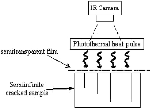
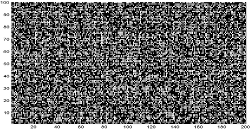
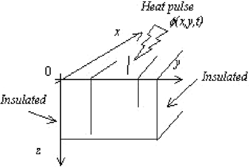
The main objective of the present work is to propose a new estimation method based on a simple experimental approach (shown in ), in order to detect the presence of cracks in the particular case where the cracks are perpendicular to the observation surface and uniform following the thickness direction. The heat pulse excitation is applied on the front face of a semi-infinite sample, with an initial constant temperature and with lateral adiabatic conditions. The spatial shape of the photothermal heat pulse has a spatially random distribution obtained by a semitransparent film inserted between the lamp and the sample (). After the heat pulse, both the lamp and the film are removed and the front face temperature field (x–y surface at z = 0) is recorded by an IR thermal imaging system. The main originality of the heating pulse is to be spatially random instead of spot-shaped or spatially uniform radiation.
In a medium with uniform properties versus z-direction and cracks perpendicular to the front surface, such as the one depicted in , the three-dimensional transient heat transfer is governed by the following general equation:
(1)
The method is concerned with the detection of cracks, which are considered as thin layers of air with a low thermal inertia. In such a situation, only a thermal conductivity variation kx(x, y) and ky(x, y) of the sample will be considered, while the volumic specific heat ρc and the thermal conductivity kz will be assumed to be uniform.
A semi-analytical quadrupole approach is then applied in order to solve equation (1) Citation9–11. Some partial spatial discretization of equation (1) is performed only versus x and y-direction, while considering the continuous variation in the z-direction. The temperature field is then represented by Tij(z, t) at N2 nodes (i, j). Performing a Laplace transformation, such as:
(2)
and introducing the vector
whose components are the Laplace-transformed temperatures
at the position z; equation (1) can be written in such a matrix form:
(3)
where M// is a finite differences operator; I the identity matrix of dimension N2; and az the constant longitudinal thermal diffusivity. The general solution of such an ordinary differential system can be presented with a function of matrix such as:
(4)
A direct relationship between the Laplace front-face temperature vector
and the Laplace heat flux vector Ψ(0,s) is found for the semi-infinite medium as Citation11:
(5)
where Z is a transfer matrix defined as:
(6)
The function of matrix used in equation (5b) is here separable by using the shift properties of the Laplace transform. If the longitudinal diffusivity az is non-uniform in the directions x and y, the problem becomes non-separable, and the approach presented earlier is no more possible, excluded as a simplified approximative method (see Citation11 for more details).
The matrix is diagonalizable such as
(7)
where Ω is diagonal matrix.
Then equation (5b) can be written as
(8)
If the excitation on the front face is a heat pulse, the components of vector Ψ(0,s) are constant and independent of the variable s, and Ψ(0,s) can be written as a constant vector Ψ0.
Since some elementary properties of the Laplace transform are considered such as the inversion of 1/s1/2 and the shift property, equation (5a) can be inverted in that case and is transformed into:
(9)
or with the exponential of matrix notation:
(10)
The averaged temperature versus x- and y-direction is now considered as:
(11)
The behaviour of ⟨T⟩ is then only related to the first eigenvalue of matrix M//, which is zero when the lateral are insulated, as considered here (see Citation11 for more details), and then:
(12)
Such a situation allows us to consider that the temperature response to any heat pulse excitation at the wall z = 0 can be expressed as the product of two separated temperature evolutions such as:
(13)
For z = 0, equation (9) becomes:
(14)
At this stage, only a simple coefficient C is considered in equation (10) instead of the exact proportionality coefficient that gives the exact temperature level, because exact IR temperature measurements are very difficult (the knowledge of emissivity, the calibration of the sensors would be necessary). This coefficient will not be taken into account in the next steps, and does not disturb the diffusivity estimation procedure, because it is removed in the estimation process.
The measured signal given by T(x, y, z = 0, t) is then replaced by a new observable variable:
(15)
corresponding to a two-dimensional signal given by the two-dimensional governing equation:
(16)
3. Implementation of the estimation method
The vector Tt corresponding to the discretization of the two-dimensional field at time t, as defined in equation (11a) is considered in the estimation process. Equation (7b) yields
(17)
For a small time step, it yields the following classical explicit expansion:
(18)
The decomposition of the finite differences matrix M// yields then:
(19)
where the operation “.*” represents the point-to-point multiplication between vectors or matrix, and
(20)
(21)
(22)
(23)
The vectors correspond to the local thermal diffusivity, and are the natural parameters of the system defined through equation (13a), obtained by spatial shifts and differences. The lateral faces are assumed to be adabatic.
From equations (13), the temperature field at time t + Δt is easily computed from the temperature field known at time t. Such an approximation is only valid if the time and space steps, Δt and Δx, are small enough for the fulfilment of the following criterion Citation12:
(24)
The estimation of the vector of parameters corresponding to the thermal diffusivity field is obtained from equations (13) by a linear autoregressive least square approach, by considering the minimization of the least-square functional S such as:
(25)
where
is an observable vector built with the difference between two successive temperature images recorded at time t = Δt amd t, such as
(26)
(27)
is the vector of parameters to be estimated, and
(28)
is the sensitivity matrix built directly with the shift and difference operations applied on the signal.
Since the measured temperature field is multiplied by the square root of time, the covariance matrix related to propagation of the measurement noise on the observable signal is proportional to the time t. Hence, the quadratic norm as defined in equation (15a) is multiplied by the inverse of the diagonal matrix built with the successive time of measurements (matrix t in equation 15a).
The minimum variance unbiased estimator of the vector β is given in that case by the maximum likelihood estimator as Citation13:
(29)
The main advantage of equation (16) is that it is built on a weighted sum of the signal which can be incremented in real time without memory storage. Even if the signal is noisy, the large amount of data allows a confident estimation of . The inversion of the information matrix
is in practice reduced to the inversion of successive small sized (3 × 3) matrices which can be implemented with symbolic computation softwares.
It is important to note that the main difficulty of the general problem corresponding to the estimation and processing of a large-sized vector of parameters is avoided. For the sake of simplicity, the ill-conditioning problems of the information matrix and other problems arising from the fact that the sensitivity matrix is built directly filled with the measured data, are not considered herein.
In the case of low-cost cameras with a very noisy signal, the main objective is to develop some rough but simple evaluation methods instead of very accurate estimation methods. In that sense, it is of interest to analyze the case where the vector of parameters is reduced to the thermal diffusivity map. Equation (15c) is then reduced to A, the sensitivity matrix is reduced to:
(30)
and the maximum likelihood estimator is given as:
(31)
The result computed from equation (18) is biased, since it is only deduced from an approximation of equation (13a). Nevertheless, such an approximation allows us to understand and to improve the experimental conditions. The very simple structure of the sensitivity matrix presented in equation (18) allows us to deduce that the best estimation conditions will occur when the Laplacian of the temperature image is maximum. Of course, the relaxation of the temperature field due to the diffusion process will be minimum or zero for long time values and maximum nearby the initial state. Thus, a uniform temperature field or a linear one in the x- or y-direction is not efficient because its Laplacian is nearly zero when the sample is homogeneous. The optimal field exists, but requires the a priori knowledge of the thermal properties field, which is precisely to be recovered. In such a situation, a spatially random initial field appears to be the best compromise, by allowing us to obtain a temperature field with a uniform spatial spectral density for initial time.
4. Some numerical examples
Some numerical experiments are analyzed. The forward method is used in order to simulate experimental data, and the estimation procedure is used for the inversion. The simulated IR images are then obtained with a division by the square root of time and a random noise addition. For the sake of clarity, only one-dimensional examples are presented in this section. Nevertheless, all the remarks given here can be extended to the two-dimensional case. Such examples will help the experimentalist to explore the limitations of the numerical processing and to design the experiment. The parameters used in these examples are very near to the real experimental conditions in the case of non-destructive evaluation for composite or metallic materials. The cracks are represented by a lower diffusivity distribution on very limited zones, generally with one pixel width. Obviously, the fracture will not be precisely located, due to the resolution limitations of the imaging system. The data chosen for this case are listed in .
Table 1. Data used for the numerical examples
4.1. Homogeneous plate – locally heated
The first example is devoted to the study of an homogeneous plate only locally heated by a heat pulse at x = 0 and z = 0. The observation of the temperature field computed from equation (13a) allows us to estimate the diffusivity field which is here homogeneous.
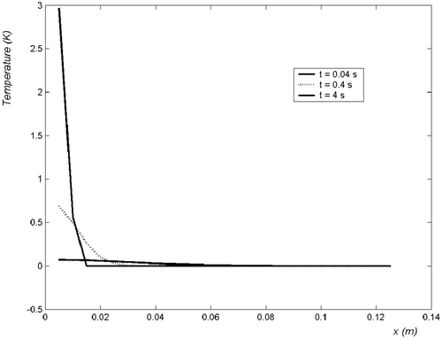
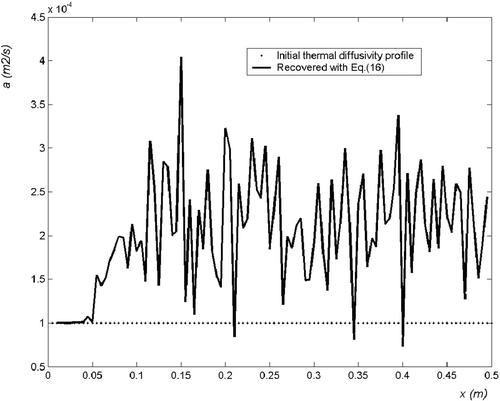
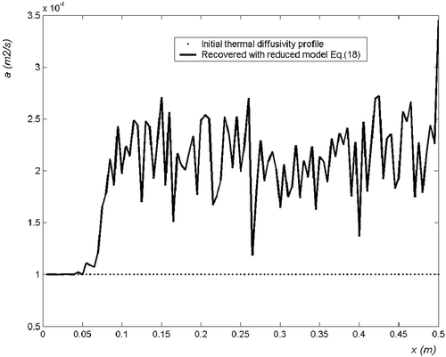
The temperature field along the medium is shown in for various values of time. The recovered thermal diffusivity field estimated from equation (16) – respectively, equation (18) – are plotted on (respectively, ). It is shown in the figures that the estimation is only efficient in a zone nearby the pertubated domain. The estimation of the theoretical diffusivity is almost perfect in the domain where the temperature gradient and Laplacian are not zero – see equations (13a) and (16). Outside of this domain, the estimation is biased, as the temperature field tends to be homogeneous. The constant bias observed outside of the heated zone is in direct relation with the uncertainity level in the sensitivity matrix. The reduced model given by equation (18) yields here a wider estimated zone than the complete model given by equation (16), since it is less sensitive to the noise.
4.2. Heterogeneous plate – randomly heated
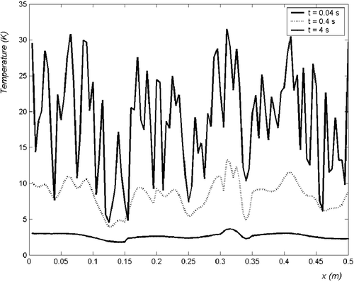
The heat pulse is spread on the whole upper surface of the plate, with a spatial random distribution (). The sample contains both a thin crack and a larger heterogeneous zone. The nominal values of the parameters are the same as in the previous example given in section 4.1, except for the noise level, which is two decades higher, with σT = 0.01 K. Some temperature distributions are shown in for various values of time, including the initial distribution given for the first time step.
The recovered thermal diffusivity field estimated with equation (16) is shown in , while is for equation (18). The estimation with equation (16) yields a better resolution but is noisier than the estimation with equation (18), which is slightly biased in the case of localized defects. Of course, such results could be greatly improved with a lower measurement noise, or a higher initial temperature field.
Figure 8. Recovered thermal diffusivity field in an heterogeneous medium with random heating; σT = 0.01 K.
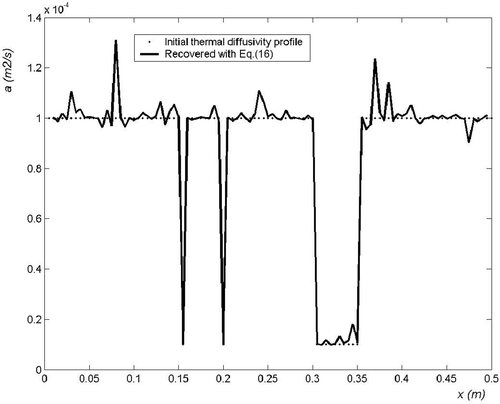
Figure 9. Recovered thermal diffusivity field in an heterogeneous medium with random heating, estimated with the reduced model; σT = 0.01 K.
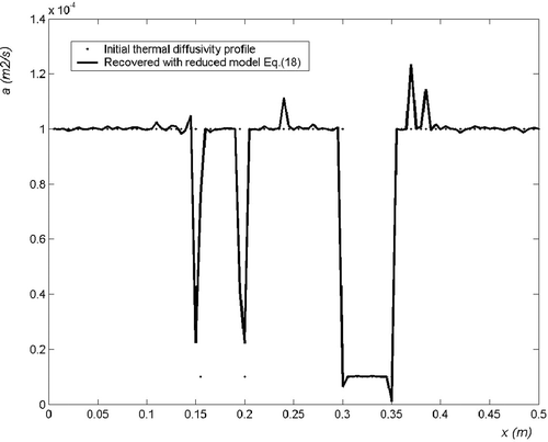
This example clearly demonstrates the practical advantage of random heating since the whole domain is pertubated. The difficulty arising with a one-spot technique is apparent in the previous example presented in section 3.1. The map estimation is made instantaneously all over the sample.
5. Conclusion
This work is an application of the semi-analytical quadrupole approach Citation9–11, which is here very helpful to demonstrate the separability of the three-dimensional temperature field, and allows us to implement an efficient inverse method from simple considerations relative to linear estimation methods.
The great advantage of such methods is to avoid memory storage and to offer a simple way to process a great amount of data related to three-dimensional heat diffusion in heterogeneous media.
It is important to point out that the experimental part of the method presented in this article has been validated in the case of thin media, where only the two-dimensional in-plane heat diffusion is considered Citation14.
Some perspectives will be to analyze (i) the experimental limitations of the proposed approach and (ii) the bias resulting from the uncertainity in the sensitivity matrix due to the fact that this matrix is directly filled with the measured data. Some other situations such as time-periodic and space-random excitation or time and space-random are also of interest.
Acknowledgments
The authors gratefully acknowledge the support of the Department of Regional Cooperation in the South Cone and Brasil at the French Embassy in Chile.
References
- Balageas, D, Delpech, JP, Boscher, D, and Deom, A, 1991. "New developments in stimulated infrared thermography applied to non destructive evaluation of laminates". In: Review on Progress in Quantitative Non-Destructive Testing. Vol. 10 A. New York: Plenum Press; 1991. pp. 1073–1081.
- Batsale, JC, Maillet, D, and Degiovanni, A, 1994. Extension de la méthode des quadripôles thermiques à l'aide de transformations intégrales-Application au défaut plan bidimensionnel, International Journal of Heat and Mass Transfer 37 (1994), pp. 111–127.
- Philippi, I, Batsale, JC, Maillet, D, and Degiovanni, A, 1995. Measurement of thermal diffusivity trough processing of infrared images, Review of Scientific Instruments 66 (1995), pp. 182–192.
- Krapez, J-C, 1999. "Simultaneous measurement of in-plane and out-of-plane diffusivity by using a grid-like mask". In: Grinzato, E, ed. Proceedings of the 5th International Workshop on Advanced Infrared Technology. Venezia, Italy. 1999. pp. 289–296.
- Varenne, M, and Batsale, JC, 2001. Infared images processing and volume averaging method in order to estimate 1D or 2D thermal conductivity fields, Image Analysis & Stereology 20 ((2) Suppl 1) (2001), pp. 299–305.
- Gruss, C, and Balageas, D, 1992. "Theoretical and experimental applications of the flying spot camera, (QIRT 92), Proc. of Quantitative Infrared Thermography (QIRT 92), Eurotherm 27, Editions Europeénes Thermique et Industrie". Paris. 1992. pp. 19–24.
- Jones, MR, Tezuda, A, and Yamada, Y, 1995. Thermal tomographic detection of inhomogeneities, Journal of Heat Transfer 117 (1995), pp. 969–975.
- Ljung, L, 1987. System Identification Theory for the User. Englewood Cliffs, NJ: Prentice Hall; 1987.
- Maillet, D, Andre, S, Batsale, JC, Degiovanni, A, and Moyne, C, 2000. Thermal Quadrupoles: Solving the Heat Equation Through Integral Transforms. New York: Wiley; 2000.
- Fudym, O, Ladevie, B, and Batsale, JC, 2002. A semi-numerical approach for heat diffusion in heterogeneous media. One extension of the analytical quadrupole method, Numerical Heat Transfer. Part B – Fundamentals 42 (4) (2002), pp. 325–348.
- Fudym, O, Batsale, JC, and Lecomte, D, 2004. Heat diffusion at the boundary of stratified media. Homogenized temperature field and thermal constriction, International Journal of Heat and Mass Transfer 47 (2004), pp. 2437–2447.
- Ozisik, N, 1988. Heat Transfer: A Basic Approach. Boston, MA: MacGraw Hill; 1988.
- Beck, JV, and Arnold, KJ, 1977. Parameter Estimation in Engineering and Science. New York: Wiley; 1977.
- Batsale, JC, Battaglia, JL, and Fudym, O, 2004. Autoregressive algorithms and spatially random flash excitation for 3D nondestructive evaluation with infrared cameras, QIRT Journal 1 (2004), pp. 5–20.
