The estimation of parameters for stochastic differential equations using neural networks

Abstract

In this article artificial neural network (ANN) is used to estimate parameters of stochastic differential equations (SDEs) given the discrete output variables of the equations. Some techniques are used to improve ANN performance in data preparation and ANN training procedure. In particular, an increase in the number of Wiener processes used to create training data set raises the accuracy of estimates significantly. The analysis of the results suggests that ANN can predict parameters of SDEs accurately under certain noise level regimes using an appropriate network architecture.

Keywords:

• Stochastic differential equations
• Parameters estimation
• Wiener process
• Artificial neural networks

1. Introduction

Some dynamic systems do not follow a strict deterministic law, and therefore stochastic models represent their behaviour more appropriately. Stochastic differential equations (SDEs) offer an attractive way of modelling the random system dynamics 1–3. An extensive list of application of SDEs in science and engineering is given by Kloeden et al. 4. As being one of the most important steps in modelling processes, estimation problems associated with the parameterised SDEs have been researched over recent decades 1, 5–7.

Artificial neural networks (ANNs) are universal function approximators that can map any non-linear function and have been used in a variety of fields, such as prediction, pattern recognition, classification and forecasting 8. ANNs are less sensitive to error term assumptions and they can tolerate noise and chaotic behaviour better than most other methods. Other advantages include greater fault tolerance, robustness and adaptability due to ANNs’ large number of interconnected processing elements that can be trained to learn new patterns 9.

The multilayer perceptron (MLP) network is among the most common ANN architectures in use. It is one type of feed forward networks wherein connections are only allowed from nodes in layer i to nodes in layer i + 1. There are other more complex neural network architectures available, such as recurrent networks and stochastic networks; however MLP networks are always sufficient for dealing with most of recognition and classification problems if enough hidden layers and hidden neurons are used 9. In this article, we use SDE parameters and their output values from the solutions of the equations to train neural networks, and use the trained networks to estimate the SDE parameters for given output data. Therefore, MLP networks will be used to solve this type of mapping problem.

The objectives of this article are to investigate the capability of MLP networks to estimate parameters of different types of SDEs, including linear and non-linear SDEs, and to identify suitable ANN model parameters, architectures and procedures to obtain optimal performances.

2. Reviews

2.1. Parameters estimation of SDE

The general form of SDE can be expressed by (1) where y(t) = the state variable of interest, θ = a set of parameters (known and unknown) and w(t) = a standard Wiener process whose increment is a Gaussian random variable with w(0) = 0, E [w(t)] = 0 and var[w(t_i) − w(t_j)] = t_i − t_j for 0 ≤ t_i ≤ t_j. All the SDEs are given in Itô forms in this article.

The first part of the right hand side of equation (1) is the drift term and the parameter μ(y, t, θ) is called the drift coefficient. The second part of equation (1) is the diffusion term and σ(y, t, θ) is called the diffusion coefficient. In practice, to determine the parameter θ, the system output variable y is usually observed at discrete time intervals, t, where 0 ≤ t ≤ T, at M independent points, where y = {y₁, y₂, … , y_M}. Observed data are recorded in discrete time intervals, regardless whether the model is described best by a continuous or discrete interval. There are various statistical methods that are used to estimate the parameters in differential equations driven by Wiener processes. An important approach is the method of moments, such as the generalised method of moments 10, the efficient method of moments 11. Another important approach is based on likelihood methods, such as maximum likelihood estimation (MLE) 12, quasi MLE 13. Among all the methods, the most commonly used one is MLE.

MLE can be used to estimate the most likely parameters for a specific SDE with a small diffusion coefficient (σ). MLE views parameters as fixed, but unknown and uncertain variables. Given a SDE in the form of equation (1) with a Wiener process {w(t), t ≥ 0} and  θ (the parameter of interest), the log likelihood ratio function of an observed path is given by equation (2), (2) The MLE of  θ may be calculated by setting the derivative of the log likelihood ratio with respect to  θ to zero and solving for θ. The major drawback is that closed form expressions for the transition and stationary probability density functions of states are not always known. For parameter estimation of non-linear SDEs, the use of MLE is, in general, not possible 6.

In this article, we demonstrate a different approach to estimate parameters of SDEs. The neural networks approach does not require the full density functions as MLE needs, nor specification of certain moment conditions required by the method of moments.

2.2. Multilayer perceptron (MLP) neural networks

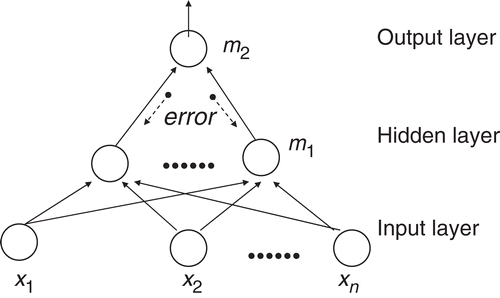
An MLP shown in figure 1 has one hidden layer (m₁) and one output layer (m₂), and all the layers are fully connected to their subsequent layer. Connections are only allowed from the input layer to the hidden layer, and then, from the hidden layer to the output layer.

Figure 1. Basic structure of an MLP with backpropagation algorithm.

The backpropagation learning algorithm was first developed by Rumelhart in 1986 14. It is commonly used to train ANNs due to its advanced ability to generalise wider variety of problems. A typical backpropagation learning algorithm is based on an architecture that contains a layer of input neurons, output neurons and one or more hidden layers; these neurons are all interconnected with different weights. In the backpropagation training algorithm, the error information is passed backward from the output layer to the input layer (figure 1). Weights are adjusted with the gradient descent method.

The ANN is trained as follows: first the network is set up with all its units and connections, and it is usually initialised with arbitrary weights. Then the network is trained by presenting examples. During the training phase the weights on connections are changed enabling the network to learn. When the network performs well on all training examples it should be validated on some other examples that it has not seen before. If the network can produce reasonable output values which are similar to validation targets and contain only small errors, it is then considered to be ready to use for problem solving.

3. Method

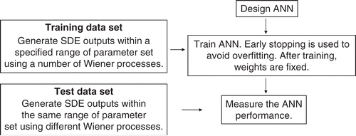
Figure 2 illustrates the outline of the procedure which includes: the preparation of training and test data sets, and feeding the data sets into ANNs.

Figure 2. An overview of the experiment approach.

3.1. Data preparation

3.1.1. Stochastic differential equations

Both linear and non-linear SDEs are examined in this research. The linear SDE [equation (3)] is expressed by a 1D diffusion equation. Its drift term has a linear relationship to the output variable of the model, and the diffusion term represents the noise in the model. Equation (4) is arbitrarily chosen as a representative non-linear SDE. (3) (4) where α, β = constant coefficients to be estimated as parameters, and γ = a constant coefficient to adjust the noise level (amplitude).

The calculation of dw(t) is as follows: the whole time span of the simulation is divided into small equal time increments, delta. dw(t) is generated using a normal distribution with the mean of zero and the SD which is equal to .

For each particular parameter α or the combination of parameters  α and β, we can generate one realisation of SDE output through equation (3) or (4). The range of  α and  β used in the experiments is 12. In addition,  γ is used to adjust the proportion of the contribution of diffusion term, and the range of  γ is [0.01, 0.1] in the linear case and [0.5, 3] in the non-linear case.

The discrete observations X(t) of these two equations are obtained at the sampling instants. Suppose the number of samples to be t_n, we consider the first t_n time steps starting from X₀ = 1 and the size of sampling interval Δt = 0.001. All the values come from the solution of SDEs. It can be shown that using Itô formula, equation (3) has an analytical solution, (5) For equation (4), we use the Euler method for the numerical solution. The numerical solution of γ = 0 has been compared with the analytical solution of the equation.

3.1.2. Neural networks data sets

Before we describe the neural network data sets, we clarify the terminology about ‘training’, ‘validation’ and ‘test’ data sets. In the literature of machine learning and neural network communities, different meanings of the words ‘validation’ and ‘test’ are employed. We restrict ourselves to the definitions given by Ripley 15: a training set is used for learning, a validation set is used to tune the network parameters and a test set is used only to assess the performance of the network.

We generate a number of SDE realisations for a specified range of parameters with some patterns of Wiener processes to train the ANN. These data sets are called training data sets and validation sets are randomly chosen from the training sets. In order to test the prediction capability of the ANN, test data sets are generated with different patterns of Wiener processes within the same range of parameters as the training data sets.

Obviously, if the test data sets were generated from SDEs which contain only a single Wiener process, the result would be biased if this Wiener process was coincidently similar to the one used to generate the training data sets. To fairly assess the performance of networks, five different patterns of Wiener processes are used to generate the test data sets.

To determine the value of time step t_n, we have taken different t_n values, where to and Δt_n = 10, to generate the training and test data sets. We found that 50 values were sufficient to represent the pattern of SDEs in order to train neural networks. Further increase in t_n did not increase the neural networks performance in parameter estimation. Therefore 50 time steps are used in our computational experiments.

3.2. Software and hardware platforms

All the experiments are carried out on a personal computer running the Microsoft Windows XP operating system. We use a commercial ANN software, namely NeuroShell2, for the neural network computations. It is recommended for academic users only, or those users who are concerned with classic neural network paradigms like backpropagation. Users interested in solving real problems should consider the NeuroShell Predictor, NeuroShell Classifier or the NeuroShell Trader 16.

3.3. Neural networks design

Among all the parameters in MLP, the numbers of input and output neurons are the easiest parameters to be determined because each independent variable is represented by its own input neuron. The number of inputs is determined by the number of sampling instants in the SDE's solution, and the number of outputs is determined by the number of parameters which need to be predicted. In terms of the number of hidden layers and hidden layer neurons, we try a network that started with one layer and a few neurons, and then test different hidden layers and neurons to achieve the best ANN performance. In the following experiments, (X − Y − Z) is used to denote to the networks, where X is the number of input nodes, Y is the number of hidden nodes and Z is the number of output nodes.

In NeuroShell2, five transfer functions are employed: logistic, linear, hyperbolic tangent function, Sine and Gaussian. We found that the logistic function was always superior to others as input, output and hidden layer functions because of its non-linear and continuously differentiable properties, which are desirable for learning complex problems. Therefore, logistic function is used in all the experiments. In addition, we use the default values of 0.1 in NeuroShell2 for both learning rate and momentum as we found that it was always appropriate.

The number of training epochs plays an important role in determining the performance of the ANN. An epoch is the presentation of the entire training going through the network. ANNs need sufficient training epochs to learn complex input–output relationships. However, excessive training epochs require unnecessarily long training time and cause over fitting problems where the network performs very well during the training but fails in testing 17.

To monitor the overfitting problem, we set up 20% of the training sets as validation sets and the ANN monitors errors on the validation sets during training. The profile of the error plot for the training and validation sets during the training procedure indicates whether further training epoch is needed. We can stop training when the error of the training set plot keeps decreasing but that of the validation set plot has an increasing or flat line at the end.

3.4. Performance measurement

In order to test the robustness of neural networks, we need to measure the level of noise in the diffusion term of a SDE with respect to its drift term. Thus, the diffusion parameter γ is used to adjust the noise level. The higher γ value indicates greater noise and increases the influence of the contribution of the diffusion term to the entire solution. As one can assume, the increased noise levels raises the difficulty of estimation. To measure it, we define P_γ for linear equation (3) as (6) and for non-linear equation (4), (7) where n = the number of time steps, and dt = time differential.

There are two parameters,  α and β, in the drift term of the non-linear SDE. We define P_α to determine the strength of the linear term [i.e. α dt x(t)]. Similarly, P_β indicates the measurement of strength of non-linear term. They can be defined as (8) and (9) R² (coefficient of multiple determinations) is a statistical indication of data sets which is determined by multiple regression analysis, and it is an important indicator of the ANN performance used in NeuroShell2 18. R² compares the results predicted by ANN with actual values, and it is defined by (10) where y = actual value,  = predicted value of y,  = mean of y and m = number of data patterns. In the case of parameter estimation for the linear SDE, one R² value is obtained for determining the accuracy of the predicted parameter α. For the non-linear SDE, two R² values are calculated for determining the accuracy of the predicted parameters  α and β. If the ANN predicts all the values correctly as the actual values, a perfect fit would result in an R² value of 1. In a very poor fit, the R² value would be close to 0. If ANN predictions are worse than the mean of samples, the R² value will be less than 0.

In addition to R², the average absolute percentage error (AAPE) is also used for evaluating the prediction performance where needed 18. The AAPE can be defined as (11) where y = target value,  = predicted value of y and m = number of data patterns.

4. Experiments and discussion

In this section, the performance of ANN is evaluated by assessing the accuracy of the estimated parameters. Different ANN architectures including various combinations of hidden layers, neurons and training epochs are used to obtain the optimum neural network. Further, a range of diffusion term is used to evaluate the effect of different level of stochasticity on the performance of ANN.

4.1. Linear SDE

4.1.1. Influence of the number of training epochs

We do not have a priori knowledge of the optimal ANN architecture at first; therefore, we choose the default parameters in NeuroShell2 for one hidden layer MLP network, which has 68 hidden neurons and the logistic transfer function for the hidden layers and output layer. In addition, α = [1, 2], Δα = 0.01 and γ = 0.03 are used for the parameters of SDE.

The experiments show that when training data set is developed using only one Wiener process, overfitting problem is obvious. To examine the effect of training epochs on average error, we plot the average error against the number of training epochs as shown in figure 3. Figure 3(a) illustrates that the average error in the training set continues to decrease during training process. Because of the powerful mapping capability of neural networks, the average error between the target and network outputs approaches zero as the training continues. Figure 3(b) demonstrates that in the first four epochs, the average error in the test set drops significantly. It reaches the lowest at the epoch 8. After that, the validation set error starts rising although the training set error becomes smaller. The reason for this increasingly poor generalisation is that the neural network tends to track every individual point in the training set created by a particular pattern of Wiener process, rather than seeing the whole character of the equation.

Figure 3. Plots of average error against epochs in the training and validation sets. (a and b): one Wiener process is used to create the training data sets. (c and d): five Wiener processes are used to create the training data sets.

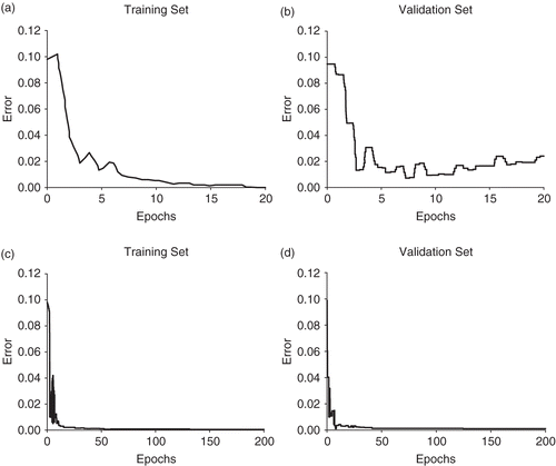
When the training data set is produced by more than one Wiener process, over fitting significantly decreases. The average error in the validation set continues to drop and remains stable after certain epochs. The average error against epochs in the case of five Wiener processes are plotted in figure 3(c) and (d). In the next section, we will examine the relationship between the number of Wiener processes and ANN prediction ability.

4.1.2. Influence of the number of Wiener processes

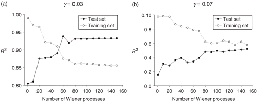
The same ANN architecture and SDE parameters as the previous section are used here. Additionally we test a set of noisier data with γ = 0.07. The results are obtained with the same numbers of training epochs. Figure 4 shows the influence of the number of Wiener processes that are used to produce training data sets. It indicates that as the number of Wiener processes in the training sets increases, the network produces higher R² values for the test sets. It should be noted that the size of training data set expands as more Wiener processes are employed, and consequently the expansion causes slower training. Therefore, although there is a marginal improvement on R² value when more than 80 Wiener processes are used, we limit the number of Wiener processes to 100 in our further investigations.

Figure 4. R² on the training and test sets against the number of Wiener processes used to produce the training sets in the case of γ = 0.03 (a) and γ = 0.07 (b).

4.1.3. Influence of the number of hidden layers and neurons

We use the same SDE parameters as in section 4.1.1 except γ = 0.07 to create training and test data sets, and 100 Wiener processes are used to produce the training data sets. All the R² values are obtained by using early stopping. The results in table 1 suggest that when there is only one hidden layer and the number of neurons in the hidden layer is very small, the performance of the network is poor because the network does not have enough ‘power’ to learn the input–output relationship. When the number of neurons in the hidden layer is close to the half number of input neurons, the performance reaches a higher accuracy. Further increase in the number of hidden layers and neurons does not improve the performance.

Table 1. R² variation on test set with different hidden neurons and hidden layers

1 hidden layer	Test set R^2	2 hidden layers	Test set R^2	3 hidden layer	Test set R^2
50-3-1	0.2728	50-3-3-1	0.5103	50-3-3-3-1	0.4920
50-10-1	0.5222	50-5-5-1	0.4916	50-5-5-5-1	0.4576
50-30-1	0.5392	50-15-15-1	0.5125	50-10-10-10-1	0.5075
50-50-1	0.5151	50-25-25-1	0.4986	50-20-20-20-1	0.4987
50-100-1	0.4980	50-50-50-1	0.4936	50-30-30-30-1	0.5072
50-200-1	0.4969	50-100-100-1	0.4669	50-100-100-100-1	0.4892

4.1.4. Influence of diffusion term

The ANN performance is investigated for different combinations of drift and diffusion terms. We use three different MLP architectures, 50-30-1, 50-15-15-1 and 50-10-10-10-1, to train and test the data sets, and record the best performance.

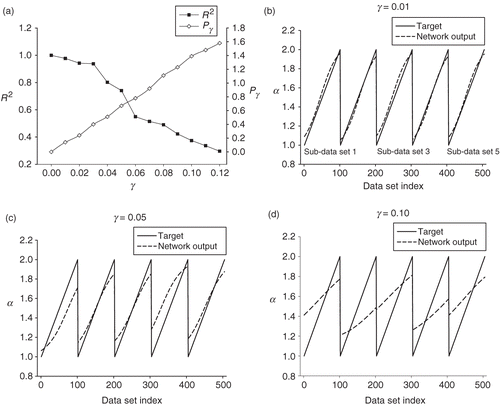
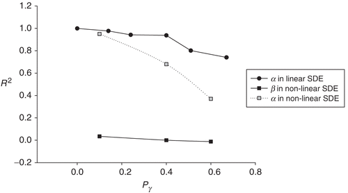
Figure 5(a) demonstrates that the ANN performance decreases as the magnitude of the diffusion term increases. Figure 5(b) shows that the target and network output in the test sets are in good agreement when γ = 0.01. Because the test set is created by five Wiener processes, it should be noticed that there are five repetitive sub-data sets and each of them represents a range of  α values, which is from 1 to 2, with one pattern of Wiener process. By observing the sub-data sets separately, we can gain a better understanding on how noise influences the estimation of the parameter. As the  γ value reaches 0.05 (figure 5c) and the ratio of diffusion term and drift term reaches 0.67 (shown in figure 5a), the 2nd, 3rd and 5th sub-data sets show more accurate predictions than the 1st and 4th sets. Figure 5(d) demonstrates that the network-generated outputs just tend to use the average of targets in most of the sub-data sets when γ = 0.10 where the weight of diffusion term is more than that of the drift term (P_γ = 1.39 as shown in figure 5a).

Figure 5. (a) The neural network performance decreases as the diffusion term in SDEs increases. (b–d) Target values and network outputs when γ = 0.01, 0.05 and 0.10; x-axis represents the index in testing data sets where five Wiener processes were used.

4.2. Non-linear SDE

In this section, we carry out similar investigations as in the linear case. Moreover, because the non-linear SDE contains two parameters, we investigate how the accuracy of estimation varies for different combination of parameters.

4.2.1. Influence of network architectures

The parameter values and ranges of the SDE are as follows: α = [1, 2], Δα = 0.05, β = [1, 2], Δβ = 0.05 and γ = 0.5. We use early stopping to find out the best results. From table 2, the different network architectures result in a very similar performance. The R² values for  α are very close to zero while the R² values for  β are all more than 0.9. According to the statistical meaning of R² explained in section 3.4, we consider that the neural networks fail to predict α and succeed in predicting β. We explore the reason for the difference between  α and  β later.

Table 2. Network performance in the non-linear SDE as network architecture changes

Network architecture	R^2 (α)	R^2 (β)	Network architecture	R^2 (α)	R^2 (β)
50-10-2	0.0256	0.9161	50-10-10-2	−0.0135	0.9209
50-30-2	0.0349	0.9453	50-20-20-2	−0.0183	0.9299
50-60-2	0.0395	0.9406	50-50-50-2	0.0134	0.9310
50-100-2	0.0296	0.9209	50-10-10-10-2	0.0128	0.9198
50-200-2	0.0354	0.9299	50-50-50-50-2	−0.0164	0.9257

4.2.2. Influence of diffusion term

We use three network architectures, 50-30-2, 50-60-2 and 50-50-50-2, to estimate parameters for different SDEs and recorded the best results. The results in table 3 indicate that the accuracy of network performance decreases as the strength of diffusion terms in SDEs increases, which is similar to the linear equation. Figure 6 shows that comparing with the results in the linear case (figure 5a), the prediction capability of networks for the non-linear case is poorer due to the complexity of input–output relationship in the non-linear SDEs.

Table 3. Network performance in the non-linear SDE as diffusion term increases

Range of α	Range of β	γ	Pα	Pβ	Pγ	R^2 (α)	AAPE (α)	R^2 (β)	AAPE (β)
[1, 2]	[1, 2]	0.5	0.12	0.88	0.10	0.0349	17.79	0.9453	4.02
[1, 2]	[1, 2]	2	0.11	0.89	0.40	0.0006	18	0.6833	9.92
[1, 2]	[1, 2]	3	0.11	0.89	0.60	−0.012	17.59	0.3687	12.96

Figure 6. The scattered graph of R² values for the parameters in the linear and the non-linear equations against their corresponding P_γ values.

4.2.3. Influence of different levels of α term and β term

To investigate the reason for largest differences in R² values for  α and β, we change the magnitudes of  α term and  β term in SDEs by altering parameters  α and  β values while keeping diffusion level an approximate constant. Table 4 shows that the bigger the contribution of a term containing a particular parameter (P_α or P_β), the smaller the error (AAPE) and better the prediction (R²) for that parameter. Therefore, we conclude that the accuracy of a parameter in a non-linear SDE is dependent on its term that contributes pro rata to the drift term.

Table 4. Network performance for different parameters in the non-linear SDE

Range of α	Range of β	γ	Pα	Pβ	Pγ	R^2 (α)	AAPE (α)	R^2 (β)	AAPE (β)
[1, 2]	[0.2, 0.4]	0.35	0.47	0.53	0.39	0.2932	13.91	0.3891	12.98
[1, 2]	[1, 2]	2	0.11	0.89	0.40	0.0006	18	0.6833	9.92
[0.8, 1.6]	[0.02, 0.04]	0.15	0.89	0.11	0.42	0.7735	8.46	0.0108	17.94

5. Conclusion

In this article, we have investigated the feasibility of parameter estimation of discretely observed SDEs using ANNs. We use some techniques to improve the ANN performance in data preparation and ANN training procedure.

In the data preparation stage, we use different time steps to solve SDEs and found 50 data points are sufficient to represent the realisation of SDEs. In addition, we emphasise the effect of the number of Wiener processes used to create training data sets. Increasing the number of Wiener processes boosts the performance of networks considerably and eliminates the overfitting problem. When overfitting occurs, the resulting network is accurate on the training set but perform poorly on the test set. When the number of Wiener processes used to generate training data sets is increased, the learning procedure finds common features amongst the training sets that enable the network to correctly estimate the parameter(s) in test data sets.

In the ANN training procedure, we use early stopping to obtain the optimum test results. We also employ different MLP architectures, transfer functions, learning rates and momentums. However, we find that these factors do not increase the performance of ANNs significantly.

The diffusion level in a SDE has a significant impact on the network performance. In the linear SDE, when the ratio of diffusion term and drift term is below 0.40, the network can estimate the parameter accurately (R² > 0.93). When the ratio reaches 0.67, the network estimates the parameter accurately only when Wiener processes in test sets and in training sets are similar. If the diffusion term is larger than the drift term, the network cannot predict the parameter(s) and only tends to give an average value of the parameters used for training data sets. For non-linear SDEs, the estimation ability of a network is generally poorer than that for the linear SDEs. Furthermore, the accuracy of a parameter in a non-linear SDE is dependent on its term that contributes pro rata to the drift term.

In conclusion, the classical neural networks method (MLP with backpropagation algorithm) provides a simple but robust parameter estimation approach for the SDEs that are under certain noisy conditions, but this estimation capability is limited for the SDEs having a high diffusion level. It should be noted that this article is an initial exploration of ANN methods for parameter estimation of SDEs and more research needs to done, for example, using recurrent neural networks and stochastic neural networks in future.

References

- Kulasiri, D, and Verwoerd, WS, 2002. Stochastic Dynamics: Modeling Solute Transport in Porous Media, North-Holland Series in Applied Mathematics and Mechanics. Vol. 44. Amsterdam: Elsevier; 2002, pp. xii, 239.
- Oksendal, BK, 2003. Stochastic Differential Equations: An Introduction with Applications. Berlin, New York: Springer; 2003, pp. xxiii, 360.
- Ottinger, HC, 1996. Stochastic Processes in Polymeric Fluids: Tools and Examples for Developing Simulation Algorithms. Berlin, New York: Springer; 1996, pp. xxiv, 362.
- Kloeden, PE, Platen, E, and Schurz, H, 1997. Numerical Solution of SDE through Computer Experiments . Berlin, New York: Springer; 1997, pp. xiv, 292.
- Watts, DG, 1994. Estimating parameters in non-linear rate equations, The Canadian Journal of Chemical Engineering 72 (1994), pp. 701–710.
- Nielsen, JN, Madsen, H, and Young, PC, 2000. Parameter estimation in stochastic differential equations: an overview, Annual Reviews in Control 24 (2000), pp. 83–94.
- Timmer, J, 2000. Parameter estimation in nonlinear stochastic differential equations, Chaos, Solitons & Fractals 11 (15) (2000), pp. 2571–2578.
- Bishop, CM, 1995. Neural Networks for Pattern Recognition. New York: Clarendon Press: Oxford University Press; 1995, pp. xvii, 482.
- Hassoun, MH, 1995. Fundamentals of Artificial Neural Networks. Cambridge: MIT Press; 1995, pp. xxvi, 511.
- Hall, AR, 2005. Advanced Texts in Econometrics, Generalized Method of Moments. Oxford, New York: Oxford University Press; 2005, pp. xii, 400.
- Ronald Gallant, A, and Tauchen, G, 1999. The relative efficiency of method of moments estimators, Journal of Econometrics 92 (1) (1999), pp. 149–172.
- Azzalini, A, 1996. "Monographs on Statistics and Applied Probability". In: Statistical Inference: Based on the Likelihood . Vol. Vol. 68. Boca Raton, New York: Chapman & Hall/CRC; 1996, pp.x, 341.
- Bibby, BM, and Sorensen, M, 1995. Martingale estimation functions for discretely observed diffusion processes, Bernoulli 1 (1995), pp. 17–39.
- Rumelhart, DE, and McClelland, JL, 1986. "and University of California San Diego. PDP Research Group , Parallel Distributed Processing: Explorations in the Microstructure of Cognition". In: Computational Models of Cognition and Perception. Vol. Vol. 2. Cambridge, Mass: MIT Press; 1986.
- Ripley, BD, 1996. Pattern Recognition and Neural Networks. Cambridge, New York: Cambridge University Press; 1996, pp. xi, 403.
- Group, WS, 2005. Frederick, MD: Ward System Group, Inc; 2005, http://www.wardsystems.com.
- Caruana, R, Lawrence, S, and Giles, CL, 2001. Overfitting in neural networks: backpropagation, conjugate gradient, and early stopping, Advances in Neural Information Processing Systems 13 (2001), pp. 402–408.
- Triola, MF, 2004. Elementary Statistics. Boston: Pearson/Addison–Wesley; 2004, pp. xxix, 838.