Abstract
The problem of image reconstruction from projections in computerized tomography, when cast as a system of linear equations, leads to an inconsistent system. Hence, a common approach to this problem is to seek a solution that minimizes some optimization criterion, such as minimization of the residual (least-squares solution) by quadratic optimization. The QUAD algorithm is one well-studied method for quadratic optimization which applies the conjugate gradient to a certain so-called “normal equations” system derived from the original system. The concept of a geometric algorithm is introduced and defined as a method that is independent of any particular algebraic representation of the hyperplanes defined by the equations. An example of a geometric algorithm is the well known ART algorithm which, when implemented with a small relaxation parameter, achieves excellent results. Any non-geometric algorithm can be converted to a geometric one by normalizing the equations before applying the algorithm. This concept, when applied to QUAD, results in a geometric algorithm called NQUAD. ART, QUAD, and NQUAD were tested on various phantom reconstructions and evaluated with respect to image quality, convergence measures, and runtime efficiency. The results indicate that NQUAD is always preferable to QUAD, thus proving the usefulness of the geometric approach. Although ART is somewhat better than NQUAD in most standard cases, NQUAD is much better when the system is strongly underdetermined (a situation corresponding to low dose radiation), and this is even more pronounced with low-contrast images.
Preliminary results presented at the 8th IASTED Conference on Computer Graphics & Imaging, August 2005.
1. Introduction
We consider the problem of image reconstruction from projections in transmission computerized tomography (CT) Citation11. After a discretization of the image domain, the problem leads to a large and sparse system of linear equations, Ax = b, which is inevitably inconsistent, due to a variety of reasons (noise, inaccurate measurements, as well as the discretization process). Solution methods usually fall into transform methods or iterative methods, with the latter being generally slower but providing superior results under adverse conditions.
Table 1. Details of the two test cases.
Table 2. Case 1—minimal distance and relative error, and iteration number(s) at which they were obtained.
Table 3. Case 2—minimal distance and relative error, and iteration number(s) at which they were obtained.
One of the earliest and most successful iterative approaches to image reconstruction from projections is algebraic reconstruction technique (ART) Citation11. In this method, originally due to Kaczmarz Citation15, each iterate is projected onto a hyperplane (defined by an equation) in a cyclic manner. ART has been studied very extensively, both in theory and in practice. It is shown in Citation11 that the addition of a small relaxation parameter into ART produces excellent results. The convergence of ART with relaxation parameters, for consistent systems, has been shown by Herman et al. Citation13 and by Trummer Citation23. Tanabe Citation22 has shown that when the system is inconsistent, ART converges cyclically, i.e., for each hyperplane, the sequence of projections on that hyperplane converges to a limit. Censor et al. Citation4 extended Tanabe's result to ART with a fixed relaxation parameter λ and also showed that for every hyperplane P, if the cyclic limit w.r.t. P is , then the limit
exists, and all the xP's coincide at a point which minimizes the (unweighed) sum of squares of the Euclidean distances to the hyperplanes. Note that such a minimization point is not necessarily unique; however, it was shown in Citation4 that if the iterations start with the zero vector, then the cyclic limits converge to a minimum norm point which achieves the above minimization.
A common approach to retrieving a “good” image is to seek a solution that minimizes some optimization criterion Citation7. One such criterion is the minimization of |Ax − b|, achieved by quadratic optimization Citation1,Citation12. |Ax − b| is the L2-norm of the residual, and a solution which minimizes this expression is also known as a least-squares solution. One way of obtaining a least-squares solution is to apply the conjugate gradient algorithm (CG) Citation14,Citation21 to one of the symmetric “normal equations” systems ATAx = ATb or AATy = b (x = ATy); see Citation2. A least-squares solution is not necessarily unique; however, there exists a unique minimum norm least-squares solution, and the iterates produced by the normal equations methods converge to this solution. Note that a point minimizing the L2-norm of the residual depends on the algebraic representation of the hyperplanes; multiplying any equation by a factor (different from zero or one) could lead to a different solution.
In contrast to the above normal equations methods, ART is a geometric algorithm in the following sense: The sequence of iterates generated by ART depends only on the hyperplanes defined by the equations and not on any particular algebraic representation of the hyperplanes. Any non-geometric iterative algorithm can be converted into a geometric one if, before applying the algorithm, the equations are normalized by dividing each equation by the L2-norm of the vector of its coefficients. This idea lies at the basis of our approach.
A simple example illustrating the difference between a geometric and a non-geometric method is the following system of two (inconsistent) equations in two variables x1,x2: x1 + 0x2 = 0 and 10x1 + 0x2 = 10. For any point x = (x1,x2), the square of the L2-norm of the residual is |Ax − b|² = x1² + (10x1 − 10)². The minimum of this quadratic polynomial is obtained at x1≈0.99. However, if the equations are normalized, then the first equation remains unchanged and the second equation becomes x1 = 1. The L2-norm of the residual of this normalized system is minimized at x1 = 0.5. This simple example illustrates how different algebraic representations of the same hyperplanes can affect the solution obtained by quadratic optimization. On the other hand, the iterates generated by ART are independent of any scaling of the equations.
In the application of CG, the literature abounds with a variety of preconditioning techniques, which can be regarded as multiplying A (on the left and/or the right) by some matrix. The particular method for quadratic optimization that we have used, which we call QUAD, is obtained by first performing column normalization on A, i.e., dividing each column of A by the L2-norm of the column, and then minimizing the residual of the resulting system Citation1. Column normalization is equivalent to right-multiplying A by a certain diagonal matrix obtained from the column norms. Note that the resulting algorithm is not necessarily geometric in the above sense, because the resulting equations are not necessarily normalized.
In this study, we apply the geometric approach to QUAD by first normalizing the equations and then applying QUAD to the resulting system. The resulting algorithm, called NQUAD (Normalized QUAD), was implemented by Mansour Citation18. Extensive experiments were carried out on many phantom images, comparing ART (with a small relaxation parameter), QUAD and NQUAD. Note Citation1, p. 245] that previous studies of QUAD did not scale the equations in any way. The comparisons employed two measures of the error (with respect to the phantom), the number of iterations required to achieve the optimal measures, and visual comparisons. Our results indicate that NQUAD is always better than QUAD on all counts, though the differences are not always visible. On an almost fully determined problem, ART produced better images than NQUAD, and in fewer iterations (though eventually NQUAD catches up).
Our most important finding is that with a strongly underdetermined system of equations (number of equations approximately equal to 25% of the number of variables) both QUAD and NQUAD were much better than ART, and NQUAD was better than QUAD. Furthermore, NQUAD achieved its best error measures in significantly fewer iterations than the other methods. Furthermore, the differences between the algorithms are much more pronounced on images of low contrast. The enhanced artifacts on low contrast images have been observed before in a somewhat different setting: “Even though these artifacts may have never been noticeable in high-contrast reconstructions, they become very visible in the low-contrast situation”— see Citation20, p. 520].
A strongly underdetermined system is compatible with a situation where low dose radiation is mandated for clinical reasons. Note that the dose is also reduced in such cases, but it is still preferable to use a technique that also requires fewer rays. Preliminary results of this research appear in Citation9.
The rest of this article is organized as follows: section 2 presents the image reconstruction problem in CT, and section 3 explains ART, QUAD, and NQUAD. Section 4 presents our results, and we conclude with some further research directions.
2. The reconstruction problem
In transmission CT, X-rays are passed through a cross section of an object and readings are taken by detectors at the opposite side. Different parts of the cross section attenuate the X-rays differently, resulting in different readings at the detectors. The problem is to reconstruct the attenuation map—or image—of the cross section from the detector readings. Mathematically, the unknown attenuation is a nonnegative function of two variables defined on the cross section. The most elementary method for reconstructing the attenuation is to overlay the cross section with a Cartesian grid of pixels, and to consider the attenuation to be constant inside every pixel. Let n denote the total number of pixels.
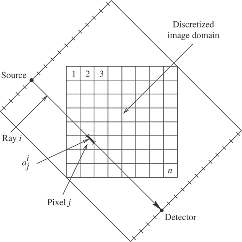
In a typical setup, we assume that a line of parallel X-ray sources are aimed at a line of detectors, as shown in . X-rays are cast toward the detectors, which measure the attenuation along the rays' paths. The orientation of the sources and detectors is then rotated by some small angle, and the process repeats until the entire cross section has been “covered” by equiangular orientations. We denote by m the total number of rays obtained in this manner.
We assume that the pixels and rays are numbered consecutively in some manner from 1 to n and from 1 to m, respectively. Let xj denotes the (assumed constant) value of the attenuation function in the jth pixel. It is assumed that the X-ray sources and detectors are points, and that the rays between them are lines. It is further assumed that the length of intersection of the ith ray with the jth pixel, denoted by represents the contribution of the jth pixel to the total attenuation along the ith ray.
The physical measurement of the total attenuation along the ith ray, denoted by bi, is the line integral of the unknown attenuation function along the path of the ray. In the discretized setup, each line integral is approximated by a finite sum, so the (discretized) attenuation function is the solution of a system of linear equations
(1)
3. ART, CG, and quadratic optimization
For , we denote by ai the ith row vector of the matrix A in equation (1). ⟨u,v⟩ denotes the dot product of two vectors u, v and |·| denotes the L2-norm of a vector, i.e., |u|² = ⟨u,u⟩. ART can be described as follows: Starting from an arbitrary point
, the k'th iterate xk is projected towards the next hyperplane, and the hyperplanes are chosen in cyclic order. We denote by i(k) the k'th index taken cyclically from 1 to m, i.e.,
. ART, with a fixed relaxation parameter λ, is the following algorithm:Algorithm 1 (ART):Initialization:
is arbitrary.Iterative step: Given xk compute
For a symmetric n × n system matrix A, the conjugate gradient algorithm is the following (see Citation21).Algorithm 2 (CG):
| i. |
| ||||
| ii. | for i = 0,1,2,… until convergence:
| ||||
| iii. | output xi. | ||||
Quadratic optimization is obtained by seeking a least-squares solution of the system (1), namely, a point minimizing |Ax* − b| (the L2-norm of the residual). It follows from Citation2, Theorem 1.2] that a solution of ATAx = ATb is a minimum-norm, least-squares solution of (1). As mentioned, QUAD applies CG to the system obtained from (1) by dividing each column of A by its L2-norm, as follows.Algorithm 3 (QUAD):
| i. | Normalize columns: For | ||||
| ii. | Apply Algorithm 2 (CG) to the (symmetric) system ETEy = ETb, obtain a solution y., and output x* = Dy*. | ||||
Our geometric approach, when applied to QUAD, transforms it into the geometric algorithm NQUAD by first normalizing the equations of (1), as follows.Algorithm 4 (NQUAD):
| i. | Normalize rows: For | ||||
| ii. | Apply Algorithm 3 (QUAD) to the system (2). | ||||
4. Results
The aim of our experiments was to provide an initial evaluation of the notion of a geometric algorithm, and how the geometric and non-geometric versions of the same algorithm differ from each other. To this end, we compared ART, QUAD, and NQUAD. There are many other reconstruction algorithms which also deserve appropriate study, and they will be the subject of future research. In ART, we experimented with different values of the relaxation parameter λ in two different ways: In one set of experiments, λ was kept fixed throughout all the iterations, and different values of λ were tested. In another set of experiments, λ was allowed to change with the iteration number in various ways. None of these experiments produced better results than a fixed value of 0.1 for λ. The comparisons between the various algorithms were made both quantitatively using the convergence measures defined in the following subsection, and qualitatively, by visual comparisons. We also tested the two parallel algorithms CAV and BICAV Citation5,Citation6, but these produced results similar to ART; they were less relevant to this study since their primary strength is in a parallel processing environment.
The three algorithms were tested on a large number of phantom test cases, with and without noise. The experiments were carried out within the framework of the SNARK93 package Citation3, which contains the means for creating various phantoms and includes a variety of standard reconstruction algorithms, including QUAD. NQUAD was implemented within the framework of SNARK93 by Mansour Citation18. In all the tested algorithms, the initial estimate was taken as x0 = 0.
Many test cases were examined, including cases with noise, and in most of these, the differences between the three methods were insignificant. Hence, we report only on cases that are relevant to the examined algorithms. These cases and the convergence measures used to compare the algorithms' behavior are detailed in the next subsection. Subsection 4.2 provides details of the results and a discussion. In subsection 4.3, we examine two more cases in order to isolate the different factors affecting the algorithms' behavior.
4.1. Test cases and measures
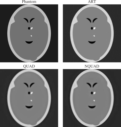
Two notable representative test cases are presented, both at a size of 255 × 255. Case 1 is the Herman head phantom Citation11, section 4.3, which is specified by a set of ellipses, with a specific attenuation value (called density) attached to each elliptical region. This phantom can be seen in . The pixel size was set identical to the inter-ray distance; this setup ensures the least amount of artifacts in the reconstructed images (as can be readily verified by experimentation). The reconstruction used 180 equidistant angles, resulting in a system of 65,025 variables and 64,980 rays—an almost fully determined system. Note that the concept of a fully determined system in CT also means that the projections are evenly distributed.
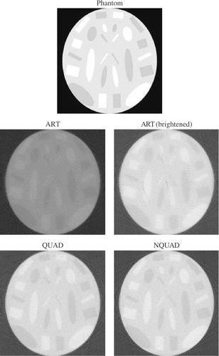
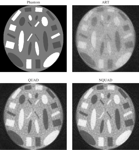
Case 2 is an example of a very adverse situation for any reconstruction method: a strongly underdetermined system of equations and a low contrast image. The phantom is based on example 7 of SNARK, modified to have very low contrast, with the low and high values differing by only 11% from the mean. This phantom can be seen in . The number of equations is only about 25% of the number of variables; this was obtained from the geometry of Case 1 by doubling both the inter-ray distances and the angle between successive projection angles. summarizes the two cases.
The values of bi, , are calculated by computing the line integrals through the elliptical regions (without reference to the discretization). Thus, the system (1) is basically inconsistent, because the left-hand-side is only an approximation to the actual integrals. This matches the real-life situation where the bi's are (path-lengths derived from) X-ray readings through an object but the region of interest is discretized as above. The algorithms were run on both cases for 40 iterations (an iteration means one cyclic sweep through all the equations).
Two measures were used to define how much a reconstructed image diverges from the phantom, the distance and the relative error. These are calculated by SNARK93 Citation3, and defined as follows. Let denote the phantom and xk denote the reconstructed image after k iterations. Let S denote the set of indices j of pixels which are in the region of interest and let α be the number of elements in S. The average value of
is defined by
and the Standard deviation of
is defined as
The distance between xk and
is defined as
Setting
, the relative error of xk is defined by
4.2. Results and discussion
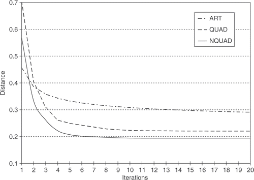
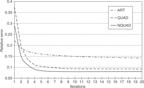
and show the minimal distance and relative error measures for the three algorithms on the two test cases, together with the iteration numbers at which the minimum values were obtained. In Case 1, the measures are not significantly different from each other, though ART reaches the minimal relative error at fewer iterations. It can be seen that ART is somewhat better than NQUAD, and NQUAD is somewhat better than QUAD; this behavior is similar in a very wide range of examples that were tested. In Case 2, the differences between the three algorithms are much more pronounced, with NQUAD having a large lead over the other two methods. Even QUAD is much better than ART in this case. Furthermore, we can see that NQUAD reached its better values relatively early. In ART and QUAD, the two measures continued to decrease till the last iteration.
and present plots of the two error measures as a function of the number of iterations for Case 2. One iteration of NQUAD took about twice the time of an ART iteration, but even so, NQUAD is clearly preferable.
, , and show the phantom and reconstructioned images for Cases 1 and 2. The images were obtained by a program called SNARKVIEW Citation8 from the output file RECFIL which is produced by SNARK93. We set this program to assign grey level zero to the lowest-valued pixel, grey level 255 to the highest-valued pixel, and all other pixels are assigned grey levels at inbetween values by linear interpolation. This method of display differs from standard practice (which assigns grey levels by considering the phantom and images together); however, it is much better at showing up artifacts in the various images. For the sake of brevity, the reconstructed images are shown only at 10 iterations.
shows the phantom and images reconstructed by the three methods for Case 1. Note that there are no visible differences between the three methods, though at 5 iterations (image not shown), ART already achieved as good an image as NQUAD at 10 iterations. shows the phantom and reconstructions for Case 2. The ART reconstruction appears dark because some pixels in the reconstructed image have a high value. We conjecture that this problem is due to the fact that ART does not deal well with the low-contrast phantom when the number of equations is small. In order to compensate for the dark ART images, also shows the ART image after it was brightened to match the general level of the other images. This was done by mapping all grey levels of 174 and above to 255, with the others linearly mapped between 0 and 255. This figure shows that the ART image is inferior to the one produced by NQUAD. The differences between the images of QUAD and NQUAD can be discerned only with difficulty.
In order to better visualize the distinctions between the reconstructions in Case 2, we applied the standard image processing technique of histogram equalization to the phantom and the reconstructed images, as shown in . Note that now the phantom no longer appears as a low-contrast image. These images reveal more strongly that ART produces some artifacts, such as the concentric “rings”, and that the various elliptical regions are not as sharply defined as in NQUAD. To the best of our knowledge, there is no mathematical explanation as to why artifacts take one particular form or another. A careful examination of the QUAD and NQUAD images reveals that the QUAD image is slightly more noisy in some places—see for example the topmost dark rectangular patch.
4.3. Intermediate cases
Case 2 differs from Case 1 in two major aspects: the number of equations is only about 25% of the number of variables, and it is of very low contrast. In view of the results of Cases 1 and 2, a natural question (raised by one of the reviewers) arises as to which of these two aspects is the primary cause of the different performance between ART and quadratic optimization. To this end, we examined two additional cases based on Cases 1 and 2:
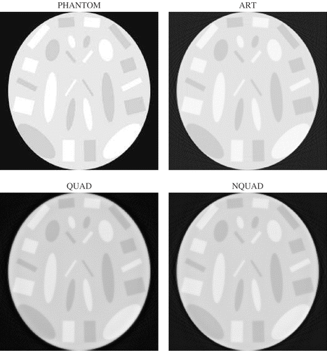
| • | Case 3: An almost fully determined system of equations (as in Case 1), but with the same low contrast as Case 2. The phantom of this case can be seen in below. | ||||
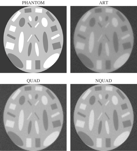
| • | Case 4: A strongly underdetermined system of equations (as in Case 2), but with an image of regular contrast. The phantom appears in below. | ||||
and 5 show the minimal measures achieved by ART, QUAD, and NQUAD for Cases 3 and 4, respectively. From we can see that (similarly to Case 1) ART performs better on an almost fully-determined system, regardless of the fact that the phantom is of low contrast.
Table 4. Case 3—minimal distance and relative error, and iteration number(s) at which they were obtained.
shows that in Case 4, with the strongly underdetermined system, both quadratic methods perform much than ART, and that NQUAD is somewhat better than QUAD.
Table 5. Case 4—minimal distance and relative error, and iteration number(s) at which they were obtained.
shows the phantom and reconstructed images for Case 3 after 10 iterations. The ART reconstruction appears “smoother” than the others, but differences between QUAD and NQUAD seem quite insignificant. shows the phantom and reconstructed images for Case 4 (strongly underdetermined system with high contrast). Both quadratic reconstructions are visibly better than that of ART, which shows some distinct artifact patterns. QUAD and NQUAD seem almost identical. However, all these differences are somewhat weaker than in Case 2 (which is of low contrast in addition to being strongly underdetermined).
Based on the convergence measures and the images, we can conclude that the major contributing factor to the superiority of the quadratic methods over ART in Cases 2 and 4 is the fact that the system of equations is strongly underdetermined. Also, under those conditions, NQUAD is somewhat better than QUAD. Furthermore, it is evident that the differences between the methods are more visibly pronounced when the data are of low contrast.
5. Conclusions and future work
This study introduced the concept of a geometric algorithm as a method (operating on a linear system) whose results are independent of any particular algebraic representation of the data. Any algorithm can be converted to a geometric one if the equations are normalized before the algorithm is applied. Quadratic optimization, in the context of image reconstruction from projections in CT, was studied by examining the QUAD algorithm. QUAD is the application of the conjugate gradient to the normal equations system derived from the column-normalization of the original system of equations. QUAD and its geometric/normalized form, NQUAD, were compared with ART (which is also a geometric algorithm) on various phantom test cases. The results can be summarized as follows:
| • | NQUAD was always better than QUAD, though the differences could not be visually detected when the equation system was almost fully determined. | ||||
| • | In an almost fully determined system, ART produced a better image than NQUAD during any given time period. However, given sufficient time, NQUAD eventually achieved the same quality. | ||||
| • | In a strongly underdetermined system, both QUAD and NQUAD were much better than ART. NQUAD achieved its optimal error measures with significantly fewer iterations (and less time) than the other two and produced images that were somewhat better than those of QUAD. | ||||
| • | The advantages of the two quadratic methods over ART are even more pronounced when, in addition to the system of equations being strongly underdetermined, the underlying data is of low contrast.The consequences are that NQUAD should always be preferred to QUAD, and that both ART and NQUAD should be readily available tools to use under different conditions. These results suggest the following directions for future research, development, and experimentation: | ||||
| • | Examination of other methods with respect to their being geometric or not. If they are not geometric, they should be compared to their performance on the normalized equations. | ||||
| • | Our discretization model assumed that throughout a pixel, the attenuation value is constant. Lewitt Citation16,Citation17 introduced a different mathematical model based on spherically symmetric volume elements, also known as “blobs”. The basis function of the pixel (or voxel in 3D) model has a value of 1 inside a unit square (cube in 3D) and 0 outside. The blob basis function is radially symmetric with a value of 1 at the center and smoothly and monotonically decreasing to zero with the distance from its center. See also Citation19 for further details. The normalization approach can also be applied to this model, and the results compared with the pixel model. | ||||
| • | Testing NQUAD in other settings that have proved to be problematic, such as cone-beam reconstructions of low-contrast objects—see Citation20. | ||||
| • | Incorporation of improved conjugate-gradient methods into image reconstruction software; see Gottlieb and Fischer Citation10. | ||||
Acknowledgments
The authors wish to thank Rachel Gordon for her help and advice. Thanks are also due to the anonymous reviewers for their helpful comments. Part of this research appeared in the second author's MA thesis Citation18 carried out under the first author's supervision at the University of Haifa.
Notes
Preliminary results presented at the 8th IASTED Conference on Computer Graphics & Imaging, August 2005.
References
- Artzy, E, Elfving, T, and Herman, GT, 1979. Quadratic optimization for image reconstruction, II, Computer Graphics & Image Processing 11 (1979), pp. 242–261.
- Björck, Å, and Elfving, T, 1979. Accelerated projection methods for computing pseudoinverse solutions of systems of linear equations 19 (1979), pp. 145–163, BIT.
- Browne, JA, Herman, GT, and Odhner, D, 1993. (1993), SNARK93: a programming system for image reconstruction from projections, Tech. Rep. MIPG198, The Medical Image Processing Group (MIPG), Dept. of Radiology, University of Pennsylvania..
- Censor, Y, Eggermont, PPB, and Gordon, D, 1983. Strong underrelaxation in Kaczmarz's method for inconsistent systems, Numerische Mathematik 41 (1983), pp. 83–92.
- Censor, Y, Gordon, D, and Gordon, R, 2001. BICAV: a block-iterative parallel algorithm for sparse systems with pixel-dependent weighting, IEEE Transactions on Medical Imaging 20 (10) (2001), pp. 1050–1060.
- Censor, Y, Gordon, D, and Gordon, R, 2001. Component averaging: an efficient iterative parallel algorithm for large and sparse unstructured problems, Parallel Computing 27 (6) (2001), pp. 777–808.
- Censor, Y, and Herman, GT, 1987. On some optimization techniques in image reconstruction from projections, Applied Numerical Mathematics 3 (1987), pp. 365–391.
- Gordon, D, 1988. SNARKVIEW–user's guide. Tech. Rep University of Haifa; 1988.
- Gordon, D, and Mansour, R, 2005. "A geometric approach to quadratic optimization in computerized tomography". In: Hamza, MH, ed. 8th IASTED International Conference on Computer Graphics & Imaging. Calgary, Alberta, Canada: Acta Press; 2005. pp. 60–65.
- Gottlieb, S, and Fischer, PF, 1998. Modified conjugate gradient method for the solution of , Journal of Scientific Computing 13 (1998), pp. 173–183.
- Herman, GT, 1980. Image Reconstruction From Projections: The Fundamentals of Computerized Tomography. New York: Academic Press; 1980.
- Herman, GT, and Lent, A, 1976. Quadratic optimization for image reconstruction, I, Computer Graphics & Image Processing 5 (1976), pp. 319–332.
- Herman, GT, Lent, A, and Lutz, PH, 1978. Relaxation methods for image reconstruction, Communications of the ACM 21 (1978), pp. 152–158.
- Hestenes, MR, and Stiefel, E, 1952. Methods of conjugate gradients for solving linear systems, Journal of Research of the National Bureau of Standards 49 (1952), pp. 409–436.
- Kaczmarz, S, 1937. Angenäherte Auflösung von Systemen linearer Gleichungen, Bulletin de l'Académie Polonaise des Sciences et Lettres A35 (1937), pp. 355–357.
- Lewitt, RM, 1990. Multidimensional digital image representations using generalized Kaiser–Bessel window functions, Journal of the Optical Society of America A 7 (10) (1990), pp. 1834–1846.
- Lewitt, RM, 1992. Alternatives to voxels for image representation in iterative reconstruction algorithms, Physics in Medicine and Biology 37 (1992), pp. 705–716.
- Mansour, R, 1999. "Geometric least squares solutions in image reconstruction". In: Master's thesis, Dept. of Mathematics and Computer Science. Israel: University of Haifa; 1999.
- Matej, S, and Lewitt, RM, 1996. Practical considerations for 3-D image reconstruction using spherically symmetric volume elements, IEEE Transactions on Medical Imaging 15 (1996), pp. 68–78.
- Mueller, K, Yagel, R, and Wheller, JJ, 1999. Anti-aliased three-dimensional cone-beam reconstruction of low-contrast objects with algebraic methods, IEEE Transactions on Medical Imaging MI-18 (1999), pp. 519–537.
- Saad, Y, 2003. Iterative Methods for Sparse Linear Systems, . Philadelphia, PA: SIAM; 2003.
- Tanabe, K, 1971. Projection method for solving a singular system of linear equations and its applications, Numerische Mathematik 17 (1971), pp. 203–214.
- Trummer, MR, 1981. Reconstructing pictures from projections: on the convergence of the ART algorithm with relaxation, Computing 26 (1981), pp. 189–195.
