Identification of point sources in two-dimensional advection-diffusion-reaction equation: application to pollution sources in a river. Stationary case

Abstract

We consider the problem of determining pollution sources in a river by using boundary measurements. The mathematical model is a two-dimensional advection-diffusion-reaction equation in the stationary case. Identifiability and a local Lipschitz stability results are established. A cost function transforming our inverse problem into an optimization one is proposed. This cost function represents the difference between the two solutions computed from the prescribed and measured data respectively. This representation is achieved by using values of these two solutions inside the domain. Numerical results are performed for a rectangular domain. These results are compared to those obtained by using a classical least squares regularized method.

Keywords:

• Inverse source problem
• Identifiability
• Stability
• Optimization
• Advection-diffusion-reaction equation

1. Introduction

When we observe a river, the transparency of its water, the natural aspect of its banks and its bottom can sometimes reflect its quality. However, to be assured of this quality, we have to analyse the composition of the water, and the quality of the sediments the river transports.

By the quality of water, we understand its physical, chemical and biological properties which can be estimated by measuring, for example, the quantity of organic matter contained in water.

By organic matter, we mean a set of organic substances that their degradation implies consumption of oxygen dissolved in water with direct consequences on aquatic life. These substances are contained in discharges of human and agricultural origin and in the numerous industrial discharges. The importance of this pollution is estimated by the measures of the so-called BOD (biological oxygen demand) and COD (chemical oxygen demand). See 12 and 13 for more details.

In order to manage and supervise efficiently the water quality in rivers, accurate determination of the location and magnitude of pollution sources is necessary.

Moreover, information regarding pollution sources is useful for addressing judicial issues of responsibility when the pollution spill is accidental or intentional.

In the present study, we are concerned with the problem of identifying the location and the magnitude (intensity) of pollution point sources from the measurements of BOD on a part of the river. The portion of the river under surveillance is assimilated to a simply bounded domain in denoted Ω with smooth boundary Γ. The governing equation and the problem statement are specified in section 2. We then prove in section 3 that the pollution sources are uniquely determined by using boundary measurements of the BOD concentration on some part Γ_out of the boundary Γ. In section 4, a local Lipschitz stability result is established. In section 5 we propose an identification method based on the so-called Kohn and Vogelius cost function for which we establish the gradient. This function is based on the energy gap between the two solutions: the first is the solution of the “Neumann” problem that considers the flux as a boundary condition on Γ_out, and the second is the solution of “Dirichlet” problem that considers the measured value as a boundary condition on Γ_out⊂Γ. Provided the data are exact and obviously compatible, we prove that the minimum of this cost function is null, and then the minimum argument is exactly the solution of our inverse problem which will be stated in the next section. Section 6, is devoted to numerical results, where some experiments are given with respect to the introduction of a Gaussian noise on the measurements and compared to those obtained using the classical least squares regularized method.

2. Governing equations and problem statement

The pollutant concentration u that we consider here (BOD) is governed by the following equations: (1) where with u the concentration of pollutant, v the mean velocity vector (v₁, v₂)^t of the river, r the reaction coefficient and F the source term. For this purpose, let γ =γ_ij denote the anisotropic tensor diffusion of the medium Ω. The coefficients γ_ij are constant and the matrix γ is assumed to be symmetric positive definite. For more information one can see 12 or 13, where detailed derivations and discussions of the governing equations for flow and transport on surface water systems are available.

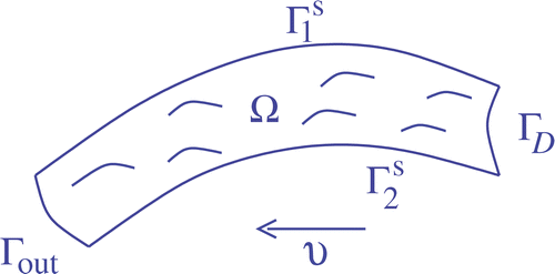
The domain Ω is assumed to be a bounded open, connected set in of sufficiently regular boundary Γ =∂Ω. The boundary Γ is assumed to be of the form , where Γ_D and Γ_N are disjoint, open subset of Γ with nonempty interior and ν denote the outward unit normal vector to Γ. Moreover, the part Γ_N is defined by with where , and Γ_out are given as follows (figure 1).

Figure 1. Polluted river.

Before starting our study, we can say here that one of the difficulties for an inverse problem regarding the identification of a function source F is the fact that we cannot uniquely determine F in its general form. We can see 8 where an example in a one-dimensional case is given and 7 for the two-dimensional case.

To overcome this difficulty, people generally assume that some a priori information on the sources is available. For example, time independent sources F(x,t)=f(x) are treated by Cannon 3 using spectral theory, and by Engl et al. 9 using the approximated controllability of the heat equation. The results of this last paper are generalized by Yamamoto 17,18 to the sources of the form F(x,t)=α(t) f(x), f∈L², where the time part function α∈C¹[0,T] is known and satisfying the condition α(0)≠ =0. Recently, Hettlich and Rundell 10 considered a 2D problem for the heat equation with the sources of the form F(x,t) = χ_D(x), where D is a subset of a disk. They proved that the set D can be identified with the measures of the flow at two different points on the boundary, and gave a numerical method to identify it. Finally, the non linear source problem, where F is dependent on the solution of the equation, that is: F(x,t) = G(u(x,t)), is considered in the papers of DuChateau and Rundell 6, and Cannon and DuChateau 4.

In our case, following the usual modeling of point sources in physics, we assume that F is of the form (2) where m is an integer, a_i are points in Ω and λ_i are scalars. Furthermore, the points a_i are assumed to be distinct.

Since the source F given by equation (2.2) belongs to the Hilbert space for s <-1, a variational formulation of the problem (2.1)–(2.2) is not possible. However, this problem is well-posed and the trace is well-defined in as we shall show subsequently. First, we define through a convolution the function (3) where E is the fundamental solution of the operator L in , that is where δ denotes the Dirac distribution at the origin. As it was known 16, E is an analytic function in , the function u₀ is also analytic in .

Let us now define the function w ∈H¹(Ω) 5 by (4) for which the trace is well-defined in . Thus the problem (2.1)-(2.2) is well-posed and then the trace is well-defined in . Then one can define the observation operator

This is the so-called direct problem. The inverse problem that we are concerned with is the following:

IP. Given the measurement , find a source F such that the solution to (2.1)–(2.2) satisfies (5)

Several questions arise in such inverse problems: does the available data f uniquely determine F (uniqueness) and if so, how does the source F depend on f (stability)? Is there a constructive algorithm for determining this source (identification)?

3. Identifiability

The identifiability issue allows us to know whether our inverse problem is well-posed in the following sense. If two measured concentrations of BOD coincide on Γ_out, then they are generated by the same source of the form (2). Furthermore, to show that the solution of the optimization problem is that of the inverse problem IP we need an identifiability result.

Our identifiability result is given by the following theorem:

THEOREM 3.1

Let , i = 1, 2. If then m₁= m₂=m, and for j=1,…,m.

Proof

Let u_i, i=1, 2 be the solutions of the following system: (6)

Assume that B[F₁]=B[F₂], we have to prove that F₁=F₂.

Consider the difference θ =u₂-u₁ which is the solution of the following system: (7)

From Holmgren theorem 14, we know that θ is identically zero in . Moreover, since with ϵ > 0, one has . Thus θ = 0 a.e. Ω which implies F¹=F² and consequently m₁=m₂=m, , and , for j=1,…,m.▪

4. Stability

In this section, we investigate the stability of our inverse problem IP. This means continuous dependence of the source F on the measurements B[F]. Stability is a crucial issue for numerical applications and it has been considered by many authors in other situations. In this section, we prove a local Lipschitz stability result derived from the Gâteaux differentiability, by establishing that the Gâteaux derivative is not null. Furthermore, we need techniques developed for stability in order to calculate the gradient given in the section 5.3.

Let . Let , which will be denoted for simplicity.

First, given and let be any vector in , then for a sufficiently small real h, .

Thus, we define the corresponding source term (8)

Let u^h be the solution to the following problem (9) and set (10)

As for the problem (2.1) the problem (4.9) is well-defined and equation (4.10) makes sense in .

Now, we are able to state our stability result given by the following theorem:

THEOREM 4.1

(Local Lipschitz stability)

If ψ≠0, then

Proof

Let . The Taylor expansion applied to F^h shows that, there exists , such that (11) with

Here denotes the second partial derivative of the Dirac distribution at point c with respect to x_i and x_j.

Therefore (12) where u¹ and u²(h) are respectively solutions of (4.13) and (4.14) defined as follows (13) and (14)

Then from equation (4.12), one deduces

First, as h is small enough, the locations are far from the boundary Γ. Then, since the distributions F¹ and F²(h) are supported respectively by {a_k} and {a_k}, , the corresponding solutions u¹ and u²(h) are well-defined, from which the traces and are well-defined in .

Moreover, according to the form of the source F²(h), and the fact that the dipole sources are well-separated from the boundary, one obtains

Then we have to prove that . That is given by the following lemma.

LEMMA 4.2

If the solution u¹ to the problem (4.13) satisfies , then ψ = 0.

Proof

By the same technique used to show identifiability, we will prove that .

Assume that , so u¹ satisfies the following system:

Using Holmgren theorem, one gets u¹=0 in . Therefore, u¹ is a linear combination of Dirac distribution and its derivatives at points a_k 15. Now, since with , . Thus, F¹=0 and then ψ = 0.▪

5. Identification

In this section, we propose an algorithm based on the minimization of a cost function of Kohn and Vogelius type. This kind of cost function has been used by many authors for various inverse problems (see for example 1,2). It indicates the energy gap between a so-called “Neumann solution” and a so-called “Dirichlet” problem corresponding to the measured data f.

5.1. Kohn and Vogelius cost function

If the source F was regular, we would have introduced the Kohn and Vogelius cost function by comparing the solutions of the problem (2.1) with Neumann condition on Γ_out and the following one

However, since the source F belongs to with ϵ > 0, the solutions of the problems (2.1) and (5.15) do not belong to H¹(Ω), so we do not proceed as mentioned above.

Nevertheless, to overcome this difficulty, we proceed in the following way.

Let u₀ be the solution of (2.3). Let w be the solution of (2.4) and the solution of the following problem (15) for which we make some variable changes in order to make this problem “symmetric”.

Let the vector κ be such that:

For simplicity of reading, we set where denotes the inner product of vector κ and X=(x,y).

Finally, we introduce the functions and which are respectively solutions of the following systems (16) and (17) where which is positive since the matrix γ is symmetric positive definite and r≥0. The cost function J is then defined as follows

5.2. Optimization problem

Consider now the following optimization problem: (18)

At first, we show that the solution of the inverse problem (2.1)-(2.2), (2.5) is the solution of the optimization problem (5.19). It leads us naturally to calculate the gradient of the functional J which will be the object of paragraph 5.3.

PROPOSITION 5.1

Let . Let be the solution of the inverse problem (2.1)–(2.2). Then ϕ is the unique element of I_ad such that

Proof

Let ϕ be the solution of the inverse problem (2.1)–(2.2), (2.5), then Thus, and therefore,

Using Holmgren Theorem, one gets z = z_d in Ω. The function ϕ is therefore a minimum of J with .

Let now ϕ₁ be another minimum for J with . Let , , , be the corresponding solutions respectively of (1), (4), (40), (44). Since , one gets, on Γ_out and then and finally . Furthermore, as and thanks to the identifiability, we get .▪

5.3. Gradient computation

Thanks to the above proposition, the inverse problem (2.1)–(2.2), (2.5) is turned into the optimization problem (5.19). Furthermore, in order to use the non-linear optimization routine optim of the scientific software Scilab (www.scilab.org), we need to compute the gradient of J, which is a vector in . To do that, it suffices to compute its Gâteaux derivative with respect to ϕ, in a direction ψ, defined as follows

First, by using the Green formula and by integrating by parts, one has which leads to

Let now F ^h in equation (4.8) be the corresponding source to . Let be the solution of problem (2.3) with F^h as source term.

From equation (4.11), we get an asymptotic expansion of with respect to the parameter h: (19) with and .

Now, set and denote z^h and the associated solutions defined respectively by, and for which one can easily derive the asymptotic expansion (20) which we need to compute the gradient of the cost function J.

Here z¹ and are respectively solutions of the following problems (21) and (22) with

Therefore, a straightforward calculation using the aforementioned asymptotic expansions (5.21) leads to

Finally, according to the condition satisfied by z on Γ_out, we obtain the following result.

PROPOSITION 5.2

The Gàzteaux-derivative of the cost function J at point ϕ in the direction ψ is given by

In order to compare the identification results obtained by the Kohn and Vogelius cost function, we also solve the identification problem by using a Tikhonov regularized least squares method. That means to minimize the following cost function with respect ϕ in I_ad where ϵ is a regularization parameter.

6. Numerical results

For numerical experiments, we are concerned with a portion of Aisne river (France) 11 assimilated to a rectangular domain Ω with a length L = 1000 meters and a width ℓ = 100 meters. We reduce Ω to and consider the following: (23) with and , , are, respectively, defined in the same manner that Γ_D, Γ_N, ν in the domain Ω. In addition, we denote by and where . Experimental measurements are simulated by synthetic data obtained by solving the problem (4), using P¹ finite elements with 20 nodes on the width of and 100 nodes on its length. These measurements are taken at the nodes of mesh on the boundary .

The gradient has been computed thanks to Proposition 2.

For numerical purpose, we consider 11, so with respect to Okubo's law 13, γ₂₂ is given by and we suppose that . For the mean velocity vector, we have where 11. The reaction coefficient is 11.

6.1. Sensitivity of the identification results with respect to a Gaussian noise

In this paragraph, we study the sensitivity of the results obtained by both identification methods, that is the first approach (Kohn and Vogelius method), developed in section 5, and the Tikhonov regularized least squares method, with respect to the introduction of a Gaussian noise on the data f. We make synthetic measurements from the source located at S=(0.643, 0.02) emitting the intensity coefficient . The results of this study are presented in table 1 below as follows: in the first column, we indicate the percentage of noise while the next two columns are devoted to the identification results obtained respectively by the first approach and the least squares method. Given a percentage of noise, we present the x-coordinate, the y-coordinate of the location S and the intensity λ identified by each method. As far as the least squares method is concerned, we consider the cost function J_LS with the geometric sequence and we choose as regularization parameter ϵ the optimal term of this sequence. The ϵ-values are represented in the last column.

Table 1. Identification with respect to percentage of noise.

Noise (%)	Kohn and Vogelius	Least squares	ϵ
0	0.645 0.0192 2.21	0.644 0.0195 2.24	0.001
1	0.647 0.0189 2.18	0.648 0.0193 2.16	0.001
2	0.638 0.0182 2.13	0.661 0.0228 2.08	0.01
3	0.631 0.0176 2.06	0.656 0.0181 1.84	0.01
4	0.657 0.0168 2.03	0.668 0.0290 1.79	0.01
5	0.671 0.0372 1.89	0.687 0.0415 1.61	0.01
6	0.693 0.0463 1.63	0.712 0.0630 1.57	0.1
7	0.707 0.0597 1.37	0.702 0.0531 1.54	0.1
8	0.731 0.0724 1.19	0.729 0.0694 1.12	0.1
9	0.786 0.0912 0.71	0.805 0.1130 0.83	0.1

In order to compare these identification results, we compute from table 1 the following mean squared errors (MSE) where and are the x-coordinate, the y-coordinate of the location S and the intensity λ obtained respectively by the first approach and the least squares method for the jth-considered percentage of noise.

The above numerical tests indicate that the identification results obtained by the first approach are better than those given by the least squares method. However, the higher intensity of noise constitutes a common limit for the two identification methods.

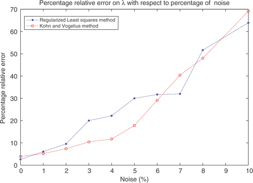
Subsequently, we present the percentage relative errors on λ, that is and for j=1,…,10 deduced from table 1 with respect to percentage of noise.

From figure 2, we remark that the Kohn and Vogelius method improves the quality of identification results especially for the lower values of percentage of noise. Indeed, the identification results given by this method are more stable than those obtained by the Tikhonov regularized least squares method with respect to the introduction of a Gaussian noise on the data f.

Figure 2. Percentage relative error on λ with respect to percentage of noise.

6.2. Case of several active sources

In this part, we compare the results obtained by the two identification methods where we consider several active sources. For these numerical tests, we introduce a fixed intensity of a Gaussian noise (percentage of noise = 3%) on the data f. The results of this study are represented in table 2 where the first column is reserved for the source from which, for each case, we constitute the synthetic measurements. The two others are reserved for the identification results given by the two methods.

Table 2. Case of several active sources.

Measure sources	Kohn and Vogelius	Least squares (ϵ=0.01)
0.227 0.092 1.47	0.216 0.086 1.28	0.203 0.077 1.19
0.841 0.069 3.25	0.834 0.060 3.11	0.827 0.058 2.98
0.100 0.001 2.43	0.079 0.002 2.18	0.053 0.003 1.96
0.617 0.098 1.65	0.608 0.084 1.46	0.602 0.076 1.38
0.832 0.034 4.12	0.838 0.043 3.98	0.821 0.026 3.74

From the numerical tests given in table 2, we remark an advantage for the Kohn and Vogelius method to improve the identification results especially in the case where the pollution has occured far from the observatory Γ_out.

7. Conclusion

In this paper, we have considered the inverse source problem of determining pollution point sources in a river by using boundary measurements. Identifiability and local Lipschitz stability results are established. For numerical purpose, we proposed a new cost function J of Kohn and Vogelius type based on the energy gap between the solutions of the so-called “Neumann” and “Dirichlet” problems for which we have proved that the unique minimum argument is the solution of the inverse problem. Several numerical tests are performed.

The comparison of the identification results obtained by this cost function J and those given by the Tikhonov regularized least squares method shows the advantage of this new identification method to improve the quality of the identification results. Indeed, the cost function J can be seen as another manner to regularize the least squares method which enables the identification results to be more stable with respect to the introduction of a Gaussian noise on the measurements and to improve them especially in the case where pollution has occured far away from the observatory.

8. Discussion

In this article, we assumed a linear advection-diffusion model for transport process and point sources. This model is also used in 8 to identify a point source and to recover its intensity function in the one-dimensional time-dependent case. As far as the applicability of this model to identify distributed sources is concerned, in 7 the authors used it to identify spherical sources where χ designates the characteristic function and ω_i the sphere centered at S_i. They also considered this model to recover a source with separated variables F(x,t)=λ (t)g(x), where the function λ is supposed known and the function g∈L₂ is unknown.

In practice the values of the diffusion and advection coefficients are largely variable from one river to another. As the precision on the numerical solution of this model depends on the transport nature: advection dominant (high Peclet number) or diffusion dominant (low Peclet number), it seems to be interesting to study the effects of the transport nature on the performance of these inverse methods. This study could be useful to identify eventual limitations of the supposed model.

Acknowledgments

This work was supported by Conseil Régional de Picardie, France for which the author expresses his sincere gratitude. Thanks is also given to the anonymous referees for their valuable comments and help.

References

- Chaabane, S, and Jaoua, M, 1999. Identification of Robin coeficient by the means of boundary measurements., Inverse problems 15 (1999), pp. 1425–1438.
- Chaabane, S, El Dabaghi, F, and Jaoua, M, 1998. On the identification of unknown boundaries submitted to Signorini boundary conditions: identifiability and stability., Mathematical Methods in the Applied Science 21 (1998), pp. 1379–1398.
- Cannon, JR, 1968. Determination of an unknown heat source from overspecified boundary data., SIAM Journal of Numerical Analysis 5 (1968), pp. 275–286.
- Cannon, JR, and DuChateau, P, 1998. Structural identification of an unknown source term in a heat equation., Inverse Problems 214 (1998), pp. 535–551.
- Dautray, R, and Lions, JL, 1987. Analyse mathématique et calcul numérique pour les sciences et techniques. Masson: Paris; 1987.
- DuChateau, P, and Rundell, W, 1985. Unicity in an inverse problem for an unknown reaction term in a reaction-diffusion-equation., Journal of Differential Equations 59 (1985), pp. 155–164.
- El Badia, A, and Ha Duong, T, 2002. On an inverse source problem for the heat Equation. Application to a pollution detection problem., Journal of Inverse and Ill-posed Problems 10 (2002), pp. 585–599.
- El Badia, A, Ha Duong, T, and Hamdi, A, 2005. Identification of a point source in a linear advection dispersion reaction equation: application to a pollution source problem., Inverse Problems 21 (2005), pp. 1121–1136.
- Engl, HW, Scherzer, O, and Yamamoto, M, 1994. Uniqueness of forcing terms in linear partial differential equations with overspecified boundary data., Inverse Problems 10 (1994), pp. 1253–1276.
- Hettlich, F, and Rundell, W, 2001. Identification of a discontinuous source in the heat equation., Inverse Problems 17 (2001), pp. 1465–1482.
- Inseba, B, 1992. Controlabilité exacte, identifiabilité, sentinelles. Thesis report, University of Technology of Compiègne. 1992.
- Linfield, C, 1987. The enhanced stream water quality models QUAL2E and QUAL2E-UNCAS: Documentation and user manual, EPA: 600/3-87/007. 1987.
- Okubo, A, 1980. Diffusion and Ecological Problems: Mathematical Models. Springer-Verlag: New York; 1980.
- Rauch, J, 1991. Partial Differential Equations. Springer: New York; 1991.
- Schwartz, L, 1966. Théorie des distributions. Hermann: Paris; 1966.
- Trèves, F, 1975. Basic Linear Partial Differential Equations. New York: Academic Press; 1975.
- Yamamoto, M, 1993. Conditional stability in determination of force terms of heat equations in a rectangle, Mathematical and Computer Modelling 18 (1993), pp. 79–88.
- Yamamoto, M, 1994. Conditional stability in determination of densities of heat sources in a bounded domain., International Series of Numerical Mathematics (Basel: Birkhäuser, Verlag) 18 (1994), pp. 359–370.