Identification strategy for orthotropic knitted elastomeric fabrics under large biaxial deformations

Abstract

Inverse methods have considerably facilitated the identification of complex responses, and hence permitted to represent more realistic behaviours. We have developed and applied a specific identification strategy in order to characterise the strongly nonlinear surface response of knitted elastomeric fabrics undergoing large biaxial deformations (>80%). These particular orthotropic materials are used for medical applications, delivering limited mechanical efforts, but which strongly depend on the fabric biaxial state of stretching. The identification procedure relies both on FE simulations using a corotational formulation, and on a full-field measurement optical method able to characterise the displacement fields under biaxial tension. A Levenberg–Marquardt algorithm is then used to identify the surface response coefficients for our fabrics, by comparing the distance between experimental and numerical results in the sense of nonlinear least-squares. This comparison requires to characterise both FE and experimental displacements/forces at the same points, which were chosen as the geometrical (fixed) points experimentally used. For the identification, several scalar and field input data were tested, it appears that the procedure is regularised by adding the global displacement comparison to the full-field displacements comparison. Eventually, the identified surfaces are shown to well-represent the fabric response for strain ranges of practical medical use.

Keywords:

• Identification
• Levenberg–Marquardt
• Digital image correlation
• Knitted fabric
• Constitutive law
• Biaxial tension
• Finite strains

Mathematics Subject Classifications::

• 74S05
• 74B20
• 74D10
• 74E10
• 74G74

1. Introduction

The identification of material parameters relying on inverse methods becomes more and more popular due to the versatility that these methods introduce in grasping complex behaviours. In turn, this permits to tend towards realistic numerical simulations, as long as the implementation remains easy and straight. This improvement is liable to the simultaneous development of new algorithms, as well as new experimental techniques that permit to provide a large amount of information to be compared with their corresponding simulated results.

Identification techniques are based now on algorithms able to handle, for large problems, the minimisation of the distance between experimental and simulated physical responses. This distance to be minimised can be expressed in various ways, the most popular being the distance in the sense of the least square 1, but other approaches exist such as the error in constitutive equation 2, the virtual fields method proposed by Grédiac and co-workers 3, or the scatter to reciprocity 4. Classically, identifications are used for physical properties 5, fed into numerical models used to generate the theoretical results to be compared with the experimental ones. But since these methods rely, very often, on experimental full-field techniques, they can also be used to detect cracks or more generally defects 2,4.

Moreover, in the case of the elastomeric fabrics studied here, the full-field measurement techniques permit to deal with large deformations, since no classical (contact) method would bear such strains. It is a peculiarity of these elastomeric fabrics which exhibit an orthotropic hyperelastic-like response, whereas in literature, textiles are characterised for small 6,7 or moderate (biaxial) strains 8,9, and rubber-like materials are isotropic 10 even under multiaxial loadings 11. These approaches have in common to rely on optical methods (12 for instance) to follow the deformation state throughout loading, but differ from our approach. Indeed, as far as the authors know, up to now no study has ever presented the mechanical characterisation, under finite strains, of the biaxial response of an orthotropic material.

In the present article, an identification strategy is proposed for determining the mechanical properties of elastomeric knitted fabrics under large biaxial deformations. This method is based on comparing experimental and calculated displacements/forces in order to minimise the distance between them. First, the identification strategy will be presented from a general point of view, outlining the difficulties to deal with and the expectations. Notably, we shall see that in the peculiar framework of the large deformations considered here, large sequences of pictures, and then sequences of loadings in the nonlinear geometrical simulations, must be considered. Then, the corotationnal formulation adopted to implement the constitutive law will be presented, followed by the choice of the strain measurement associated with it. Briefly, the experimental characterisation will be summarised, and after evaluation of the efficiency of the procedure using 1D generated results, the identification will be applied on our knitted fabrics under large biaxial stretching.

2. Identification strategy

Since our material is to be characterised under finite strains, the identification must be adapted to the nonlinear comparison of parameters. Several techniques are good candidates for this type of identification, for instance Kalman filters 13 would be appropriate here. But in the scope of our material properties identification, we have preferred a Levenberg–Marquardt algorithm 14, a robust first order method able to locate local minima for nonlinear least squares. Although the CPU identification time can be high with this method, it has the advantage of being already implemented in ZéBuLon® 15, an object-oriented F.E. solver which provides moreover a meta-language very useful to implement owner's material formulation.

2.1. Convergence criteria

The identification of a constitutive law by an inverse method is based on the determination of the theoretical material parameters which yields the best fit of some experimental measurements, in the sense of the postulated physical model. This operation requires the definition of the objective function which measures the difference between the experimental data and the corresponding theoretical values. Equation (1) gives the expression of this function for two vectors of data (1 × N), in the sense of least squares as used by Levenberg–Marquardt14 : (1) where y_theo(J_i) are the simulated results generated with a set J_i of material coefficients, and y_exp are the experimental values. The data vectors must represent the physical quantities at the same locations x and same instants t for the comparison to be proper and are classically normalised to yield unit-independent results.

From this objective function, the Levenberg–Marquardt minimisation process 14 calculates the local gradient by finite differences to evaluate the scaling vector t_i that modifies the set of parameters J_i. For every new set of simulated results, the minimisation convergence criterion is mainly 2-fold exclusive 15. A simple comparison of the objective function with a fixed convergence tolerance ε is tested first (equation 2), as can be applied numerically. A small value of ε is qualified as a severe criterion of convergence and will certainly lead to an increase in the cost (time) of the identification: (2) Second, the change in the new set of parameters (J_i+1=J_i+t_i·J_i) must be significant, i.e. larger than a fixed scalar value δ:

(3)

After one of these criteria is passed, the algorithm will test the stability of the solution obtained. The problem is then solved for sets of parameters in which every coefficient is successively perturbed (scaled in the research space axis), this permits to detect the existence of local minima in the vicinity of the optimum coefficient set, i.e. for which the objective function is smaller: . If the stability test fails for a coefficient set, the minimisation process restarts from this new point . Only after this test is fully passed will the algorithm stop and provide the best fit of parameters J 14.

2.2. Dealing with large biaxial deformations

The fabrics considered exhibit an orthotropic nonlinear reversible behaviour under large strains as detailed subsequently (section 3). Regarding the identification of such constitutive behaviours, Hartmann et al. 10 propose a method to identify the constitutive law of carbon black-filled rubber specimens based on the measurement of the contour of the sample and following various points plotted on the specimen. The authors succeed in identifying the material parameters of a hyperelastic isotropic model, classically based on a potential formulated as function of the principal stretches. In our study, the orthotropic behaviour plus the large stretches undergone by the compressible fabrics do not permit to easily write such a potential. Nevertheless the principle can be applied to our fabrics, with the advantage to have access to full displacement fields through digital image correlation where the tracers of the motion are the out-of-plane rugosities of the fabrics. Obviously, forces and displacements on the edge of the specimen are also accessible in the tension experiments carried out.

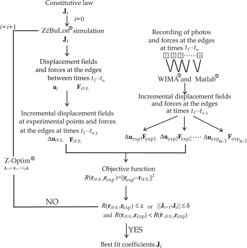
Eventually, the identification of the nonlinear material behaviour relies on a classical identification scheme, except that here complete loading sequences have to be considered since large strains are encountered. The whole identification algorithm is easily visualised on the diagram presented in figure 1, and the main stages of the identification are as follows:

i.	Acquisition of pictures and forces at the edges at times t1, …, tn.
ii.	Digital image correlation to extract incremental displacements (WIMA® software 12), and forces processing (Matlab®) at times t1, …, tn−1.
iii.	Choice of a constitutive law–set of coefficients Ji where i = 0. a. Finite element simulations (ZéBuLon®) of a biaxial tension test using coefficients Ji. b. Objective function: measure the difference between experimental rexp and simulated riF.E. displacements and boundary forces for the complete sequence, i.e. for times t1, …, tn−1. c. Test for convergence and stability: d. While convergence and stability fail, run steps (a) to (d) with a new set of coefficients (Z-Optim) ELSE issue best fit coefficients Ji.

Figure 1. Identification diagram of a nonlinear constitutive law under finite strains.

The diagram of identification (figure 1) shows that one can dissociate two essential branches. A first branch is related to the experimental part (right-hand side in figure 1) which comprises the acquisition of the picture sequence, the recording of the forces at the edge of the sample, and their treatment to extract two sets of information: displacement and forces at each time t_i ∈ [t₁, …, t_n−1] which form the vector r_exp. These data are measured at fixed time increments corresponding to the time increment between two consecutive picture shots. The second branch of the identification diagram corresponds to the calculation part which is made up mainly of nonlinear F.E. simulations. From these computations one can deduce the nodal incremental displacements of the F.E. mesh and the edge forces of the sample, which form the vector r_F.E.. At that stage, in order to compute the objective function, it is necessary to compare the same quantities at the same times (loading) and locations. For the loading, the F.E. loading steps are taken as the experimental loading steps corresponding to the image shot times t₁, …, t_n−1. As for the location, the F.E. mesh nodes do not correspond to the centres of the windows used to calculate the displacement through the digital image correlation technique. A further C++ program permits to deduce the F.E. displacement at these geometrical points using the nodal displacements and interpolation functions, once the geometrical point has been located in the F.E. mesh.

3. Experimental and numerical specificities in the case of knitted elastomeric fabrics

The knitted elastomeric fabrics studied here are used as medical compression stockings in the treatment of veinous deficiencies 16. These articles are used under large deformations, indeed the European pre-norm 17 prescribes that these compression stocking articles must be able to withstand more than 120% of deformation without any degradation. Generally, two types of knitted elastomeric fabrics are considered for stocking articles (figure 2). The structure with a course (inlaid) reinforcement (figure 2a) was considered in this work, it is named Diaphane 2 by Ganzoni which produces it, it was already used for stocking studies 16. In figure 2(a) the loops of the knitted structure which ensure the cohesion of the article can be seen and are used as a support for the inlaid yarn inserted in the course direction.

The peculiar architecture of the considered fabrics induces an orthotropic behaviour, i.e. characterised by constant mechanical properties in orthogonal symmetry planes. Only two orthotropy planes are of interest here, they are normal to the fabric plane and orientated along the course and wale directions (figure 2), the third plane in the fabric thickness being of no interest since fabrics are used for their in-plane properties. Moreover, as it is a characteristic for membranes to poorly respond under shear loadings, only tensile properties are considered here.

Figure 2. Knitted structure of medical compression stockings: (a) inlaid knitted structure (b) floatted structure.

As for large strains, they can be obtained by the use of Lycra® for the core of both loop and inlaid yarns, then covered by polyamide fibers used to increase the dyeing potential of the fabric without altering the sensitivity of the mechanical properties of the yarn. Very few studies presented in the literature actually deal with a material behaviour which could be close to this nonlinear elastic orthotropic behaviour. Hyperelasticity would be a good candidate to represent our fabrics response, since textiles usually exhibit a J-type response, i.e. a tensile response nonlinear for low strains followed by a constant tangent stiffness and eventually by hardening at high strains (see 18 for instance). This hardening is in hyperelastic rubbery materials due to the orientation of macromolecules, while it is due to the loops locking in fabrics. Unfortunately, knitted fabrics have not been studied much from a mechanical point of view, except for their use for reinforcements in composites 7,19–21. One can however cite a work by Itskov and Aksel 22 who proposed a model for orthotropic hyperelastic materials. But this model is rather heavy to handle, and most importantly, all the hyperelasticity approaches rely on the hypothesis of (quasi) incompressibility, which is not the case in our material. On the contrary, this incompressibility will introduce severe numerical problems (23 for instance), while it is not at all essential here.

One can verify that our orthotropic viscoelastic knitted fabrics undergoing large deformations cannot be characterised very easily through classical approaches. Specific experimental and numerical approaches have then been developed.

3.1. Experimental part

3.1.1. Material used

The mechanical response of our elastomeric fabrics is characterised by a low stiffness along with a viscous (delayed) response induced by the use of Lycra®. Moreover, the knitting plus the inlaid (course) yarn yields an intrinsic biaxiality of the response.

The knitted fabrics visco-elastic response was then characterised, since polymeric cores are used for both inlaid and loop yarns. These experiments were carried out on narrow bands of fabrics, 200 × 30 mm² (transverse direction × loading direction), which permit to ensure a constant stress state in the loading direction 24. Both stress and strain relaxation tests were carried out on Diaphane 2 which showed that the characteristic relaxation time is about 6 min. This was confirmed by tensile tests carried out for various displacement rates which did not show any loading rate sensitivity for regular rates.

3.1.2. Experimental tests

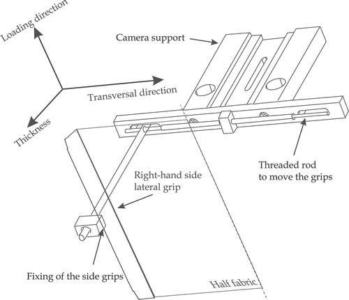
Our experiments aim at measuring the biaxial response of the knitted elastomeric fabrics. This is achieved, on a simple tension machine, thanks to the device presented in figure 3, modified by special guide bars adapted on the clips to induce transverse tension (figure 4).

Figure 3. Experimental device for biaxial-induced tension equipped with the camera–pantograph system.

Figure 4. Device for transversally induced tension. Only one lateral grip is represented.

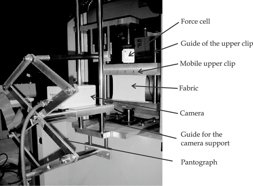
The principle of this device, in its uniaxial version (figure 3), is to induce a tensile loading in fabrics. Special care has been brought to the gripping (or clipping) of the fabrics which are quite fragile and can easily tear off. In this device, a camera used to take the picture sequences is mounted on a pantograph which permits to target the centre of the specimen all along the loading, and independently from the stretching of the fabric. This gives us a fixed reference for the displacement measurements deduced with the digital image correlation technique.

In its biaxial-induced tension version, the device is equipped with some guides, referenced as ‘lateral grip’ in figure 4, around which the fabric is tied and stapled, but can still freely move vertically. The idea here is to take advantage of the high ‘transverse shrinkage’ under tension 20,21,25 characteristic of knitted fabrics. By maintaining the transverse dimension, a transverse tension is induced. Then, uniaxial tests are repeated for various fixed transverse dimensions, and eventually yield a set of biaxial test results.

As for the measured data, pictures are taken with a camera CCD HAMAMATSU C4742-95-12NRB of a resolution of 1.3 million pixels (1024 pixels horizontally and 1280 pixels vertically). The maximum frequency of the picture acquisition is of 10 images per second. Acquisition is managed by a software developed under IMAQ® by National Instrument, named VisionStage. The tensile force in the loading direction is recorded simultaneously by means of a program written under Labview®. This force recording is subsequently treated so that forces are known at the same instants that pictures are taken.

3.1.3. Digital image correlation technique

Very briefly, digital image correlation techniques rely on the comparison of the grey levels contained in pictures representing two states of the same medium. The versatility, but at the same time the difficulty, of the method consists in comparing solely the grey levels in both pictures without any further consideration about geometry or behaviour. In fact, this comparison is achieved in subdomains called windows, where a scalar measure of the grey level (sum, scalar product, …) that they contain is defined. Then, windows are taken sequentially in the first picture, a measure of the grey levels is calculated in every window, and the closest window is redsought black in the second picture. Closest means in the sense of a least difference in terms of grey-level measure. This technique was developed for fluids flows 12,26,27, but can be easily extended to any field of application as soon as particles can be traced between images. Obviously, some limitations exist which are related to the definition of vicinity for the grey-level measure: at least two-thirds of the particles must be common between two windows in a pair of pictures. In our case, this will set the time increment between the image shots, also considering the window size defined in pixels, the camera capacity, the machine loading rate and the precision expected.

As for the tracers, the fabric surface irregularities (figure 2) are used as natural grey-level contrasters. But since we deal with large deformations, not only a pair of pictures is used, but a whole sequence of pictures is analysed. The displacement field is determined incrementally, i.e. by considering two consecutive images of the sequence. Then, owing to the fixed reference targeted by the camera, the relative (incremental) displacement field can be obtained for every couple of images: it corresponds to the displacement field undergone by the material points between two loading increments.

3.2. Calculation part: finite element simulations of the biaxial tension tests

Since large deformations are expected for our experiments, the F.E. simulations must account for geometrical nonlinearities: finite strains and rotations. Moreover, a specific constitutive law has to be fully implemented, it will naturally account for any rotation of the orthotropy axes, i.e. will be formulated in a corotational framework.

The environment used for the simulations is ZéBuLon®, a full-featured nonlinear F.E. solver with many special abilities for material-oriented analysis. The solver has been shown to be effective for very large nonlinear problems, both in terms of number of degrees of freedom, and number of convergence increments required. ZéBuLon® provides a meta-language which is very useful to implement one's material formulation or element. Moreover in this code some optimisation facilities are incorporated in the Z-Optim® toolbox. Globally, for our application ZéBuLon® offers the possibility to easily implement a specifical constitutive law, while providing the required tools to identify the parameters of this constitutive law.

3.2.1. Corotational formulation

As it is usually the case in versatile open F.E. codes, when requiring user material analyses ZéBuLon® transfers to the user the responsibility of properly writing the mechanical formulation of the equilibrium. The user must then chose a strain measure and the conjugated stress, and provide both secant and tangent material constitutive matrices, all these quantities being written in the proper referential accounting for potential principal axes rotations.

For finite strains, several alternatives exist in formulating the mechanical equilibrium. Mainly, this depends on the volume over which the integrals are computed, and on the choice of the strain measure. ZéBuLon® provides several ways to define the strain measures starting from the deformation gradient, noted F(x,t) 15. Strains can be, for instance, computed from the deformation gradient polar decomposition which writes: (4) with R(x, t) an orthogonal second order tensor associated with the material pure rotation, i.e. rotations of the principal axes of deformation, and U(x, t) associated with the pure stretch ratios, i.e. the stretch written on the reference configuration.

In the so-called Eulerian formulation, the Cauchy stress tensor σ_loc(x,t) is related to the logarithmic strain tensor {ln [U(x,t)]{ through a constitutive law represented with the corresponding nonlinear material stiffness tensor , it writes : (5) which has to be transformed in the global framework of representation through rotations, and accounting for the volume change, to deal with global quantities: (6) This last rotation transformation (equation (6)) may be of major importance, since our fabrics cannot withstand shear while a local material rotation can induce ‘apparent global’ shear if the proper rotations are not achieved. Such rotations may occur when free edges are considered, as in uniaxial tests for instance, or very locally in biaxial tension when stretchings are not equilibrated in both directions. Moreover, as it is classical for orthotropic materials, it was assumed that in our tension-dominated models, the orthotropy axes remained normal, i.e. no squeezing of the material axes could occur. The rotation was then applied to the course direction where the inlaid yarn induces the stiffest behaviour.

This corotational formulation, along with two others (see 24 for details) was validated on a simple shear test. This severe test corresponds to large shear strains for a single linear isoparametric F.E. element under plane stress ruled by a linear isotropic constitutive law. Results obtained correlated perfectly the benchmark tests proposed by Forest 28. An Eulerian formulation was chosen, since it permits to achieve vanishing shear stress for large strains, i.e. for a flattened element. This is important for our fabrics which cannot withstand shear, it validates the chosen formulation which can be used to model the biaxial tension tests.

3.2.2. Tensile tests simulations

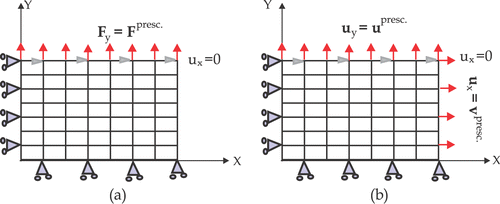
The tensile tests used for the identification were modelled with 8-noded bi-quadratic isoparametric finite elements in plane stress, regarding the very thin fabrics used. Uniaxial and biaxial tests were simulated under finite strains. Due to the loading and kinematical boundary conditions symmetry, only a quarter of the specimen was modelled. Simulations were carried out under ZéBuLon® with some level of loading corresponding to the various instants of image shots, as explained earlier. In figure 5 the corresponding boundary conditions are schematically depicted, with prescribed forces and displacement in 1D, but displacements prescribed purely in 2D. This choice corresponds to the most easily accessible experimental data for both cases.

Figure 5. Tests simulations: (a) uniaxial tension case, (b) biaxial tension case.

In the identification procedure, selected data are used to build the data vector r_iF.E. in figure 1. After every run, mesh nodes coordinates and forces at the edges are recorded. From the node positions, the displacement of the geometrical points (centres of the windows in the digital image correlation method) is calculated through a C++ program. For the isoparametric quadrangle finite elements used, this consists of determining with the ‘capable angles’ method the element to which the considered point P belongs 29. Briefly, this consists of forming four triangles with point P and every pair of nodes, then the sum of the angles at summit P will be 2π if P belongs to the element, and 0 if P is located outside. When the element is located, displacement shape functions of this element are used to rebuild the displacement at point P in the reference element, and eventually project in the real space to get the displacements of point P.

3.3. Validation of the identification procedure applied to a F.E. generated cases

Before using the identification for the knitted fabrics response, the identification procedure was validated using generated data for uniaxial tests. This validation was carried out for accuracy, since target coefficients are known, but also the robustness was evaluated by verifying that different starting parameters would not change the final results. This was done systematically even if not reported henceforth. This validation also permitted to evaluate the CPU costs as functions of the convergence tolerances, and to select the results used to form the data vectors. Results of uniaxial tests were generated by a ZéBuLon® finite element model. This model represented a simple tension test with 35 loading steps, and a mesh comprising 2200 dofs in total. A Mooney–Rivlin incompressible hyperelastic constitutive law was used, described through a potential expressed in terms of principal stretch ratios: (7) where the C_ij's are the material parameters, and I₁ and I₂ are, respectively, the first and the second invariant of the Cauchy–Green tensor. The third invariant I₃ corresponding to the volume variation is null for fully incompressible materials. In order to simplify the calculations, only coefficients C₁₀, C₂₀, C₂₁, C₀₃ were considered. The corresponding constitutive law is plotted in figure 6 for values of the coefficients reported in table 1. As it is classical for textiles, stresses in the fabric plane have no meaning regarding the fabric thickness variability, and are consequently replaced by forces per unit width.

Figure 6. Uniaxial hyperelastic response used to generate F.E. results for the identification validation. Mooney–Rivlin coefficients given in table 1.

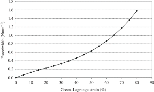
Table 1. Mooney–Rivlin target and identified coefficients under uniaxial tension comparing: only upper edge position, only displacement fields, and both simultaneously.

	C10	C20	C21	C03	CPU time [h]
Target coefficients	50.02	−8.27	10.1	−0.050
Edge position	50.00	−8.27	10.0	−0.190	4	3.69 · 10^−11
Displacement field	50.00	−8.27	10.0	−0.088	94	3.2 · 10^−10
Edge position & Displ. field	50.00	−8.27	10.1	−0.102	52	3.68 · 10^−10
CPU times and objective function terminal values are also reported.

3.3.1. Choice of the type of data used for the identification

The first type of data used to identify the response was the fabric upper edge displacement, corresponding experimentally to a displacement of the tension machine cross-head. The solution is obtained after 4 h of calculation (CPU time) on a pentium PIII 1.2 GHz processor. This corresponds to 101 computations/iterations with tolerances ε (equation (2), absolute objective function tolerance) set to 10⁻¹² and δ (equation (3), parameters change tolerance) to 10⁻⁵. Iterations ran between convergence, at iteration 52, and the end of the identification process correspond to some tests of the stability of the best fit obtained, as it can be seen on the oscillations of coefficient C₀₃ in figure 7. In this identification process, the objective function is 3.69 × 10⁻¹¹, this means that the optimisation process stopped due to sets of parameters which could not be modified to decrease the objective function, i.e. the criterion of equation 3 was passed. The influence of the convergence tolerance ε on the CPU times and results accuracy was tested subsequently.

Figure 7. Change in the Mooney–Rivlin material parameters and error vs. the optimisation iterations for upper edge position comparison.

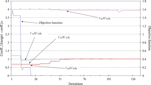
For the present identification, the identified coefficients are very close to those used to generate the ‘experimental’ results, except for coefficient C₀₃ which remains different from the exact solution (figure 7 and table 1). This difference could be explained by the little influence of this parameter on the constitutive law (equation (7)).

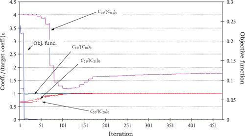
Secondly, the material coefficients were identified by comparing the displacement fields inside the specimen. This approach is similar to the experiments that were planned to be achieved to identify the behaviour of our knitted fabric. The identification CPU time is in this case much more important than the former relying only on the upper edge displacement. It is about 94 h, the parameters that minimise our problem are reached after 451 iterations. Despite the higher cost of this approach compared to the previous one, the coefficients identified are more accurate (see the Objective function scale and coefficient C₀₃ in figure 8), although the objective function is 3.2 × 10⁻¹⁰ ‘only’. But once again, the convergence tolerance ε is quite severe here.

Figure 8. Change in the Mooney–Rivlin material parameters and error vs. the optimisation iterations for displacement fields comparison.

Eventually, a combination of displacement field and edge displacement was considered. The identification procedure needs in that case 52 h to converge. It is an intermediary time between the two other approaches (4 and 94 h). The solution was reached after 241 iterations (figure 9) with an accuracy slightly improved (see C₂₁ and C₀₃ in table 1).

Figure 9. Change in the Mooney–Rivlin material parameters and error vs. the optimisation iterations for upper edge position and displacement fields comparison.

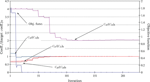
In table 1 the coefficients values obtained when using the three methods are presented. It comes out that comparing local data, such as the displacement field, yield an improved accuracy but a large CPU amount. When comparing also the global (edge) displacement, times are reduced by a factor 2 while the accuracy is acceptable. In fact, in a more realistic case, the CPU amount has to be reduced further. Let us evaluate the effect of the convergence tolerance on both result accuracy and CPU times.

3.3.2. Influence of the convergence tolerance on the CPU times

As it is often the case, a balance must be found between the CPU times and the result accuracy. As shown in figure 10, the CPU times for identification comparing upper edge displacement and displacement fields decreases almost linearly according to tolerance ε. On the other hand, the identified parameters change significantly only when an error of <10⁻² is prescribed. As a conclusion, a reasonable accuracy can be expected with a tolerance in the range [10⁻⁴–10⁻⁶].

Figure 10. Change in the identification CPU time vs. convergence tolerance ε–comparing both displacement fields and upper edge position.

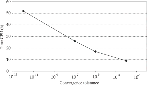
Observing the CPU resources used during the identification procedure, it appeared that most of the calculations were required to form the objective function obtained through an internal Linux command (i-file-file type). It was decided to integrate the comparison of the files and the estimate of the objective function, in the sense of nonlinear least squares, into our program C++ used to process the ZéBuLon® results rather than carry out these calculations with the Z-optim module. In that way, the CPU time was reduced by a factor 2, as shown in table 2.

Table 2. Changes in CPU times required for comparing vector files with internal ZéBuLon® functions and using owners' C++ program.

Convergence tolerance ε	CPU time ZéBuLon® internal function [h]	CPU time owners' program [h]
10^−2	9	5
10^−5	17	7
10^−7	26	12
10^−12	52	27

Eventually, comparing both local and global displacement permit to achieve the coefficients identification in a quite reasonable amount of CPU time, while yielding a good result accuracy. This was also verified on a biaxial test generated set of results 24, which showed to yield proper identified parameters with some CPU times around 80 h for 14 material coefficients and a 24,000 dofs mesh. Most notably, it appeared that differences in stiffness between course and wale directions induced some problems in properly identifying both responses, especially for low strains. This appeared also, obviously, for the real fabric as described subsequently.

4. Identification results and discussion

4.1. Surface response

The validated identification procedure was then used for knitted elastomeric fabrics undergoing biaxial finite strains. Regarding the difficulty in representing the peculiar behaviour of our orthotropic nonlinear knitted fabrics, it was decided to use a surface response to be implemented subsequently in F.E. codes 30. This solution has the advantage of remaining simple enough, even for orthotropy, without returning to very heavy formulations such as suggested for instance by Itskov and Aksel 22, especially as the behaviour considered here is not ‘fully’ orthotropic but more biaxial in tension. Boisse et al. 30 used this method to represent the behaviour under forming processes of various composite materials with woven carbon fibre reinforcement. For orthotropic cases, two different surfaces have to be used, one for the course forces (F_C) and the second one for the wale forces F_W which both depend on course (ϵ_C) and wale (ϵ_W) strains. Formulas (equation (10)) present the expression of the models of the forces in wale and course directions that are to be identified : (8) where a_i's, b_i's, c_i's, and d_i's, are coefficients to be determined. In both formulas the ‘Poisson's’ effect was modelled by a second-order polynomial function. Stresses and strains are related through a sixth-order polynomial in the course direction, and a fourth-order polynomial function in the wale direction. In total, 14 coefficients have to be identified.

4.2. Results/discussion

As explained previously, the experimental test consists of inducing a transverse tension by restraining the fabric deformation transversally to the stretching induced by the machine. The experimental details of these tests are given in table 3. For the calculation part, a quarter of the fabric was modelled with 120 2D isoparametric elements in plane stress with a quadratic interpolation. These simulations reproduce the experiments, leading for every set of constitutive material parameters respectively to 4 and 5 F.E. models for the 150 × 150 mm² and 110 × 110 mm² tests, each composed of 28 and 21 loading steps, respectively (table 3).

Table 3. Experimental data of the biaxial tensile tests.

Length × width (mm × mm)	110 × 110	150 × 150
Loading rate (mm/min)	200	200
Scaling (mm/pixel)	0.061	0.062
Image number	28	21
Image frequency (s^−1)	1.3	0.816
Transverse dimension (mm)	0, 20, 40, 70	0, 10, 30, 50, 70

In these experiments, the transverse tension is induced by prescribing different transverse dimensions (table 3). Since a single cell force is used, the experiment is made twice for the force recording: the upper edge displacement being in the wale direction and then in the course direction. Globally, this yields almost ‘symmetrical’ stretchings for the fabric, although the real use in medical compressive stockings is more uniaxial, with about 30% in the wale direction against 80–120% in the course direction.

4.3. Discussion

4.3.1. Experimental results

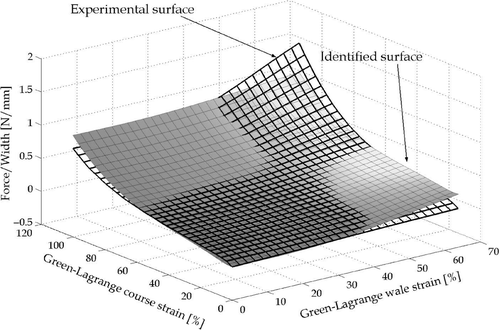
Two series of experiments were carried out with two specimen sizes, 150 × 150 mm² and 110 × 110 mm², leading respectively to Green–Lagrange [Course]∩ [Wale] strain ranges of [0,45%]∩ [0,35%] and [0,100%]∩ [0,65%]. Figures 11–14 show the experimental and identified response surfaces for both specimen dimensions. Let us first observe the experimental results corresponding to the grid-dots data in these figures. For the 150 × 150 mm² specimen, the course and wale forces appear to depend on both course and wale strains, relatively linearly for the course force (figure 11) and in a J-like manner for the wale force (figure 12). This is in accordance with the course-reinforcement of the fabric which transforms the J-like response, characteristic of knitted articles, into a more homogeneous solid-like response in this direction for strains lower than 40%. For larger strains (figures 13 and 14), up to 100%, the course force depends mainly on the course strain (figure 13) while the wale force depends mainly on the wale strain (figure 14), both in a J-like manner. However for large course and wale strains a stiffening effect induced by stretching in the normal direction appears, particularly for the course force (figure 13).

Figure 11. Change in the course force vs. wale and course strains for the 150 × 150 mm² knitted fabric.

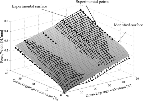
Figure 12. Change in the wale force vs. wale and course strains for the 150 × 150 mm² knitted fabric.

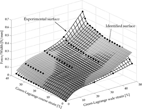
Figure 13. Change in the course force vs. wale and course strains for the 110 × 110 mm² knitted fabric. Strains of practical interest are bonded with the solid line.

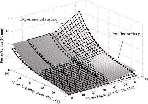
Figure 14. Change in the wale force vs. wale and course strains for the 110 × 110 mm² knitted fabric. Strains of practical interest are bonded with the solid line.

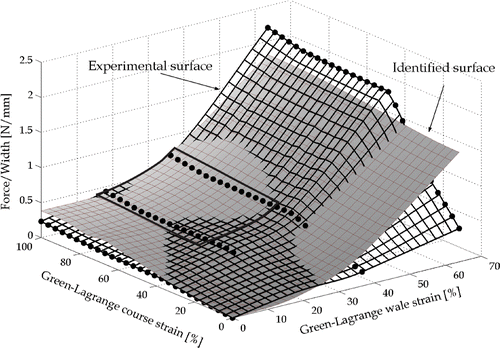
It must be pointed out that for these extreme loadings, the fabrics deteriorate due to tears. In fact these loadings are out of the European pre-norm 17 which stipulates course strains up to 120% but wale strains of about 30 to 40% ‘only’. For these strains of practical use ({ϵ_C,ϵ_W}∈ {[60%, 100%], [20%, 40%] }), schematically represented in figures 13 and 14, one verifies that the course yarn reinforcement induces a course response which depends on course strains only, while the wale force is weaker and depends mainly on the wale strains. This is the effect sought in medical compression stockings: the course reinforcement, i.e. the compressive effect, depends mainly on the stretching in the leg circumference equal to the ratio of stocking to leg circumferences. Conversely, the wale strain which corresponds to pulling on the stocking cloth, has no significant effect on the pressure delivered by the medical compression stocking.

4.3.2. Identification and error estimate

Let us now observe the identification processes, the characteristics of which are presented in table 4. One can notice that the value of the objective function is rather important, it reveals some difficulties in fitting the experimental values, which consist of displacements and forces, with the proposed response (equation (10)). The identified parameters for the 110 × 110 mm² case are shown in table A1. In order to evaluate the difference between the experimental and identified surface, an error is defined which measures the relative distance between the two responses: (9) where N is the number of experimental measurements, and et are, respectively, the identified and experimental forces per unit width at experimental point i. It must be pointed out that for low experimental strains, this error will increase, but most of the identification problems arise for large strains.

Table 4. Details of the identification procedure applied on knitted fabrics 110×110 mm² and 150×150 mm² for a polynomial response model (equation 8).

Specimen (mm^2)	Total iterations	Convergence iteration [#]	CPU time [h]	Objective function
150 × 150	216	197	11	15.9
110 × 110	202	183	4	401.45

Figure 15 presents the variation of the relative error for the course force for the 110 × 110 mm² case. The average value is 0.218 while it is only 0.074 for the 150 × 150 mm² case. For the wale response, the average value is a bit greater than for the course one, it reaches 0.313 (figure 16) against 0.152 in the 150 × 150 mm² case. But this error is in fact heterogeneously distributed, for small and large strains. Considering strains of practical use, as defined previously, yields some errors of 0.084 and 0.079 for the course and wale response respectively (table 5). Clearly, as shown schematically in figures 13 and 14, this region of practical strains is the one for which the identified surface properly fits the experimental response (see also dotted-line region in figures 15 and 16).

Figure 15. Error on the course force vs. wale and course strains for the 110 × 110 mm² knitted fabric. Strains of practical interest are bonded with the dashed line.

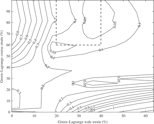
Figure 16. Error on the wale force vs. wale and course strains for the 110 × 110 mm² knitted fabric. Strains of practical interest are bonded with the dashed line.

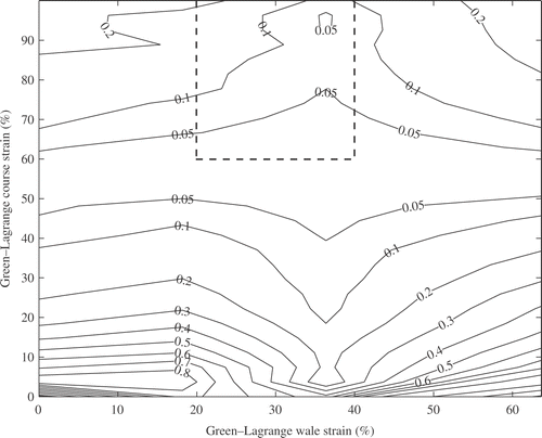
Table 5. Error as defined in equation 9 for the various identification results, considering the whole range of strains and for practical strains.

		110 × 110 14 coeffs.		110 × 110 24 coeffs.
Identif. test	150 × 150 [0,45] ∩ [0,35]	[0,100] ∩ [0,65]	[60,100] ∩ [20,40]	[0,100] ∩ [0,65]	[60,100] ∩ [20,40]
FWale	0.152	0.313	0.079	0.35	0.082
FCourse	0.074	0.218	0.084	0.19	0.085

In order to make sure that the difference between identified and experimental results, especially at large strains, is not due to the fact that only a second order polynomial function is used to represent the transverse effect, identification calculations have been processed with a sixth order polynomial function to integrate the transverse phenomena. In this case 24 coefficients are to be identified (table A1). The value of the objective function this time is quite large, and the average error for the wale force is 0.35 and 0.19 for the course force. As shown in figure 17 the results do not change significantly. For the practical strains, the mean error reaches 0.082 and 0.085 for the wale and course forces, respectively (table 5), exactly as for the 14 coefficients case.

More generally, regarding the objective function value and the error measured, it was demonstrated that improving the polynomial representation of the constitutive law (surface response) considered may be unlikely to bring a form able to represent the local effects, especially for large strains. This is quite normal, regarding the very different responses in wale and course directions that the same constitutive law has to represent. Only a mean response can be identified, even with a surface description improvement or a reduction in the optimisation tolerances.

Anyway, as explained previously, in their nominal use these fabrics withstand strains of about 30% in the wale direction against 80–120% in the course direction. In our case, for both large wale and course strains, a fabric degradation appears, the test is too severe. Identification of the surface response on a more restrained experimental domain can be considered, since in addition a rather ‘light’ surface response has to be provided for computational purposes. This is reinforced by the mean error which decreases by more than a decade, from 0.2–0.3 to 0.08 when these practical strains are considered. As a conclusion, the present identification methodology has to be refined for unsymmetrical loadings, i.e. [60%, 120%] for the course and [10%, 50%] for the wale direction. This depends mainly on the testing device which has to be equipped so as to characterise wale and course forces in the same test.

5. Conclusion

Specificities of our knitted elastomeric fabrics used under large biaxial deformations led us to develop and apply a dedicated identification procedure. The experimental part is based on a specific biaxial-induced tension rig equipped with a pantograph to support a CCD camera. This camera is used to take picture sequences which are processed through a digital image correlation technique that yields the incremental displacement fields acting in the specimen during the complete loading path. The second part of the identification procedure consists of FE models including a fully nonlinear formulation in ZéBuLon® framework, and a Levenberg–Marquardt optimisation procedure which controls the minimisation of the distance between experimental and computed data vectors.

After validation of both experimental and computational procedures, the identification has been tested on generated 1D and 2D cases. It appeared that distributed as well as global data should be considered to improve the identification accuracy, while speeding up the process. Then this identification methodology was applied to real elastomeric fabrics under biaxial stretching. Experimental results revealed that when both course and wale strains are large, the fabric exhibit very stiff responses. The identification of the surface response showed that some pronounced local effects appear under large strains which cannot be represented easily, mainly for two reasons. First, the course reinforcement yields two different behaviours in course and wale directions, and second for high strains the fabric knits tend to get locked. It results that only a mean response can be obtained which was shown to be sufficient for strains met in practical use. Indeed, the use of these fabrics in medical clothes do not involve such high combined stretchings, since only the course response is of medical interest.

Appendix

Here (table A1) the coefficients of the polynomial form are given (equation (8)) representing the surface response of 110 × 110 mm² fabric, using 14 coefficients and 24 coefficients. These results correspond to the surface responses plotted in figures 11–14, and 17.

Figure 17. Change in the course force vs. wale and course strains for the 110 × 110 mm² knitted fabric with 24 coefficients identified.

Table A1. Coefficients of the response surface identified by ZéBuLon® for the 110 × 110 mm² fabric using 14 and 24 coefficients for the polynomial representation (equation (10)).

Coeffs of the response surface (equation (8))	14 coefficients	24 coefficients
aa	70.781	−27.292
aa	−126.617	106.541
aa	106.487	−100.764
aa	−43.830	41.150
aa	9.507	−6.235
aa	−0.120	0.873
ab	−	1.016
ab	−	1.027
ab	−	1.032
ab	−	0.966
ab	1.965	0.245
ab	−0.363	0.050
ac	−	1.561
ac	−	1.987
ac	1.985	−0.140
ac	42.173	20.931
ac	−15.072	−0.018
ac	2.217	−0.031
ad	−	0.029
ad	−	−0.536
ad	−	−1.008
ad	−	−0.444
ad	0.250	1.780
ad	0.452	0.006

References

- Tikhonov, AN, Goncharski, AV, Stepanov, VV, and Yagoda, AG, 1995. Numerical Methods for the Solution of Ill-posed Problems. Boston: Kluwer Academic Publisher; 1995.
- Bonnet, M, and Reynier, M, On the estimation of the geometrical support of modelling defects using the distributed error in constitutive equation. Presented at Proceedings of Inverse problems, Control and Shape Optimisation. Carthage, Tunisia, 8–10 April, 1998.
- Grédiac, M, 2004. The use of full-field measurement methods in composite material characterisation: interest and limitations, Composites Part A–Applied Science and Manufacturing 35 (7–8) (2004), pp. 751–761.
- Bui, D, and Constantinescu, A, 2006. Spatial localization of the error of constitutive law for the identi-cation of defects in elastic bodies, Archives of Mechanics 52 (2006), pp. 511–522.
- Constantinescu, A, 1995. On the identification of elastic moduli from displacement-force boundary measurements, Inverse Problems in Engineering 1 (1995), pp. 293–315.
- Stumpf, H, Lenz, T, Schulte, K, and Andersson, CH, 1999. The mechanical behaviour of single-tricot warp-knitted fabrics: Part I: an experimental investigation of knitted fabrics of varying loop geometry under tensile stress with special attention given to inter-yarn friction, Journal of the Textile Institute Part I: Fibre Science and Textile Technology 90 (2) (1999), pp. 209–224.
- Pandita, SD, and Verpoest, I, 2003. Prediction of the tensile stiness of weft knitted fabric composites based on X-ray tomography images, Composites Science and Technology 63 (2003), pp. 311–325.
- Boisse, P, Borr, M, Buet, K, and Cherouat, A, 1997. Finite element simulations of textile composite forming including the biaxial fabric behaviour, Composites Part B-Engineering 28 (4) (1997), pp. 453–464.
- Milani, AS, and Nemes, JA, 2004. An intelligent inverse method for characterisation of textile reinforced thermoplastic composites using a hyperelastic constitutive model, Composites Science and Technology 64 (2004), pp. 1565–1576.
- Hartmann, S, Tschöpe, T, Schreiber, L, and Haupt, P, 2003. Finite deformations of a carbon black-filled rubber. Experiment, optical measurement and material parameter identification using finite elements, European Journal of Mechanics A-Solids 22 (3) (2003), pp. 309–324.
- Chevalier, L, Calloch, S, Hild, F, and Marco, Y, 2001. Digital image correlation used to analyze the multiaxial behavior of rubber-like materials, European Journal of Mechanics A-Solid 20 (2) (2001), pp. 169–187.
- Ducottet, C, Faurnel, T, Courbon, M, Moine, M, and Schon, JP, Logiciel WIMA. France, 2002.
- Bolzon, G, Fedele, R, and Maier, G, 2002. Parameter identification of a cohesive crack model by Kalman filter, Computer Methods In Applied Mechanics and Engineering 191 (25–26) (2002), pp. 2847–2871.
- Le Riche, R, and Guyon, F, Least squares parameter estimation and the Levenberg–Marquardt algorithm: deterministic analysis, sensitivities and numerical experiments. France, 1999.
- "Zébulon 8.5. Z-set Version 8.5, 2003, Transvalor/ENSMP". B.P. 87, 91003 Evry cedex, France: Centre des Matériaux, and Northwestern Numerics Inc., 150 Nickerson Street #102, Seattle, WA 98109, USA.
- Gaied, I, Drapier, S, and Lun, B, 2006. Experimental assessment and analytical 2D predictions of the stocking pressures induced on a model leg by medical compressive stockings, Journal of Biomechanics 39 (2006), pp. 3017–3055.
- Technical Comity CEN/TC205, 2001. "Medical compression stockings". In: European pre-norm. European Comity of Normalization CEN; 2001.
- Postle, R, Carnaby, GA, and De Jong, S, 1988. The Mechanics of Wool Structures. New York: Ellis Horwood Limited; 1988. pp. 195–273, Chap. 9, 10.
- Huang, ZM, Ramakrishna, S, Dinner, HP, and Tay, AAO, 1999. Characterization of knitted fabric reinforced elastomer composite, Journal of Reinforced Plastics and Composites 18 (2) (1999), pp. 118–137.
- Huang, ZM, Ramakrishna, S, and Tay, AAO, 2000. Modeling the stress/strain behaviour of knitted fabric reinforced elastomer composite, Composites Science and Technology. 60 (2000), pp. 671–691.
- Luo, Y, and Verpoest, I, 2002. Biaxial tension and ultimate deformation of knitted fabric reinforcements, Composites Part A-Applied Science and Manufacturing 33 (2002), pp. 197–203.
- Itskov, M, and Aksel, N, 2004. A class of orthotropic and transversely isotropic hyperelastic constitutive models based on a polyconvex strain enregy function, International Journal of Solids and Structures 41 (2004), pp. 3833–3848.
- Zienkiewicz, OC, and Taylor, RL, 2000. Finite Element Method, . Vol. 1. Elsevier; 2000, The Basis.
- Gaied, I, 2004. "Contribution á l étude de la contention : Approche bidimensionnelle, Identification du comportement biaxial en grandes déformations des tricots élastomériques". France: École Nationale Supérieure des Mines de Saint-étienne; 2004, PhD thesis.
- Gommers, B, Verpoest, I, and Van Houtte, P, 1996. Modelling the elastic properties of knitted-fabric-reinforced composites, Composites Science and Technology 57 (6) (1996), pp. 685–694.
- Willert, CE, and Gharib, M, 1991. Digital particle image velocimetry, Experiments in Fluids 10 (1991), pp. 181–193.
- Westerweel, J, Draad, AA, Van, Der Hoeven, GT, and Van Oord, J, 1996. Measurement of fully-developed turbulent pipe flow with digital particle image velocimetry, Experiments in Fluids 20 (1996), pp. 165–177.
- Forest, S, 1996. "Modeles mécaniques de la déformation hétérog‘ene des monocristaux". France: École Nationale Supérieure des Mines de Paris; 1996, PhD thesis.
- Gardan, Y, 1988. Élément de CAO: Matériels et Logiciels de Base. Vol. 1. Paris: Hermes; 1988.
- Boisse, P, Gasser, A, and Hivet, G, 2001. Analyses of fabric tensile behaviour:determination of the biaxial tension-strain surfaces and their use in forming simulations, Composites Part A-Applied Science and Manufacturing 32 (10) (2001), pp. 1395–1414.
Appendix
Here () the coefficients of the polynomial form are given (equation (8)) representing the surface response of 110 × 110 mm2 fabric, using 14 coefficients and 24 coefficients. These results correspond to the surface responses plotted in figures , and .