Numerical analysis of a calibration problem for simulating electric fault arc tests

Abstract

In this article, we present a mathematical model and a numerical approach for a computer-based simulation of electric fault arc tests including the solution of corresponding direct and inverse problems. In particular, we replace the complicated initial-boundary value problem of heat transfer in arc tests by a one-dimensional model based on a purely time-dependent temperature function G(t) of hot gas in a neighborhood of the arc. We analyse the forward problem with respect to its well-posedness and suggest an appropriate numerical approximation. However, we are especially interested in the ill-posed nonlinear inverse problem of identifying (calibrating) the important parameter function G from temperature measurements at a defined distance to the arc during some time interval, where a simplified test procedure is exploited for obtaining temperature data. We present a least-squares solution indicating the ill-posedness effect by strong oscillations and compare a solution from Tikhonov regularization with a solution from a descriptive regularization approach.

Keywords:

• Parameter identification
• Electric fault arcs
• Initial-boundary value problems
• Ill-posedness
• Regularization
• 2000 Mathematics Subject Classifications
• 35R30
• 65M30
• 65J20

1. Introduction

Fault arc tests are performed in textile research and certification of protective clothes. The protective clothes we are concerned with are used by people working on electric installations who are exposed to the risk of fault arc accidents, potentially causing injury with heavy burns. There exist different international standards for arc tests on such protective textiles 8. One particular European test is the so-called CENELEC test, prescribed in the pre-standard ENV 50354:2001. This box-arc test method 11 contains a visual assessment (after flaming, hole formation, shrinking, etc.) as a qualitative criterion and was extended and improved by including additionally a quantitative measurement of temperatures in order to get information about transmitted energy. A schematic test arrangement of such a complemented test is shown in figure 1.

Figure 1. Schematic test arrangement.

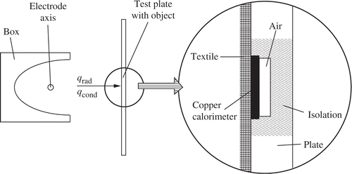
An electric arc is fired between two vertically arranged electrodes in a test circuit of defined voltage (AC). After the burning-time interval of t_p = 0.5s the arc is switched off. A surrounding box focuses thermal arc effects in direction to a test plate with test object, which is arranged in a defined distance to the electrodes. The object consists of a variable number of textile layers stretched onto the test plate and a skin-simulating copper calorimeter embedded by an isolating block in the test plate as shown in figure 1. The calorimeter is connected to a thermocouple, and so the calorimeter temperature is measured from the arc ignition (t = 0) until the end of measuring time t^end=30s.

Such tests are expensive to realize, and extensive technical equipment is required. A current of 7 kA has to be controlled and held stable in a circuit for half a second, the complete arrangement has to sustain temperatures of several thousand degrees. Moreover, the textile or clothing which is tested will be destroyed during the test. For these reasons large series of arc tests, for instance in order to take parametric studies, are not practicable. This gives rise to the need for a model of the test which enables us to study the influence of some material parameters on thermal test results.

A numerical simulation of calorimetric arc effects based on the complemented test method was realized at Chemnitz University of Technology in cooperation with the Saxon Textile Research Institute (STFI) and Ilmenau University of Technology 12. The underlying model, proposed in this article, is based on the following assumptions:

•	A nonlinear heat equation is set for the heat flux inside the object (textile and calorimeter). An important part of the nonlinearities takes the radiation which is modeled inside the object by a special source term.
•	For modeling the boundary conditions a heat transfer proportional to the temperature difference at the interesting material borders is assumed.
•	Both boundary conditions and radiation source include a simulated gas temperature G, modeling the influences of hot gas between the arc and the examined object. Unfortunately, this temperature as function of time is unknown. The reason for this holds in the high, fast changing temperatures and the explosion effects caused by the arc. The used measuring device is not able to determine this temperature (nevertheless, exactly seen G is only a model quantity and so cannot be measured).

Thus, in order to use the model we need the function G. Its determination is proposed in the following manner:

•	We focus on a special case, the test without textile layers.
•	Temperatures on the back side of the calorimeter can be measured for this test. This way, measurement data is available.
•	The determination of the unknown temperature function G by using this data leads to an inverse problem. Studying it in several aspects is the main part of the article.

This article, which is an extended version of 13, will be organized as follows: for the numerical simulation of the test we used a mathematical model, which will be described in section 2. In the model-building process, we have replaced the very complex structure of the system formed by arc, heated gas, and reflecting box by a gas temperature function G depending on time t only. The determination (calibration) of this parameter function G, which influences the result of test simulation in an essential manner, leads to the inverse problem discussed in this article. Before handling the stable approximate solution of this inverse problem in sections 5 and 6, we briefly analyze the associated forward problem in section 3 and discuss its numerical solution in section 4. We end with some conclusions in section 7.

2. The mathematical model

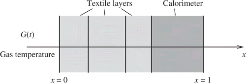
We have simplified the whole test arrangement in form of a locally one-dimensional heat equation problem, where the gas temperature near the arc is assumed to be a function G(t) of time t. The spatial x-axis lies orthogonal to the surface of the test object (plate with or without textile) such that the temperature of interest here are directed along the x-axis. Figure 2 shows the modeled object with three textile layers as an example.

Figure 2. 1D-model of the object.

We use the following notations:

x	=	1D local coordinate, x∈(0,l),
t	=	time, t∈[0, tend],
u = u(x,t)	=	temperature in the object,
G = G(t)	=	temperature of the hot gas,
CA(x,t,u)	=	apparent heat capacity (modified, specified by volume),
κ (x,u)	=	thermal conductivity,
frad(x,t,G,D)	=	radiation heat source term,
h0, hs	=	heat transfer coefficients.

The occurring temperatures u and G are seen as relative temperatures with respect to the ambient temperature T₀=300 K. Moreover, we define the space–time cylinder Q:=(0,l)×(0, t^end).

Then, the temperature distribution u=u(x,t) is the solution of the initial-boundary value problem for the heat equation, (1) with boundary conditions (2) (3) and initial condition (4) Heat effects enter the model by boundary conditions in form of heat convection and by the source term f_rad in the differential equation indicating the effect of radiation. We formulate the corresponding forward problem.

Definition 2.1 

(Forward problem) Let the parameters C^A, κ, h_s, h₀, G and f_rad be given. Find a solution u of (1–4) in .

Note, that the source term contains a special nonlinearity. In particular, f_rad depends only on the temperature u(0, t), t∈ [0, t^end], at the left boundary. Standard theory of quasi-linear differential equations presumes, that f_rad is a function of the temperature u itself. Therefore, we briefly consider conditions for the solvability of the problems (1–4). We assume for the gas temperature that with and a given maximal gas temperature G_max. Here, C[0, t^end] denotes the Banach space of all continuous functions on the interval [0, t^end]. Moreover, for the coefficients C^A and κ we assume for all that (5) with constants , and κ₂. Then we can prove the following existence result in the space , which contains all functions on , which are twice continuously differentiable with respect to the first and once continuously differentiable with respect to the second variable.

PROPOSITION 2.2 

Let and let the inequalities (5) hold. Moreover, we assume that for all for some constant C > 0 and for some constant which depends on i = 1, 2 and t^end. Then there exists a solution of (1–4).

Sketch of a proof 

We consider the mapping , where M(u₀) is the solution of (1–4) when u is replaced by u₀ in the coefficients C^A and κ and in the source term f_rad. Since we consider a linear parabolic initial boundary value problem, the mapping M is well-defined (see, e.g., [10, Theorem IV.5.4] for an existence and uniqueness result). Moreover, by [10, Theorem I.2.3] we have the estimate where and depends only on , i = 1, 2, and t^end. If we introduce the set , then M maps Ω into itself. Moreover, is uniformly bounded in the norm of [10, Theorem IV.5.3]. Hence, by the well-known compactness of embedding from into , the range for any bounded subset is relatively compact in . Thus, M is a compact operator. By Schauder's fixed-point theorem (e.g., [16, Theorem 2.A]), M contains a fixed-point which solves (1–4).▪

Recalling the technical background, the recommended continuity of the function G is not very restrictive with respect to the model.

In order to calculate u(x, t) from (1–4) the knowledge of the gas temperature G(t), t∈ [0, t^end], is required. For the determination of this function, temperature measurement data from calibration tests are used. The calibration test is performed without textile layers, where the object consists of the test plate with the calorimeter only. For this reason, we use the simplified version (6) of heat equation. Here the volumetric heat capacity C_Cu and the thermal conductivity κ_Cu are assumed to be constant. Note that κ_Cu in fact depends on the temperature, but the measured and simulated temperatures of the copper calorimeter are from the temperature interval [20,110° C] (see section 6). For this range, however, the thermal conductivity of copper is nearly a constant (e.g., [9, Chapters 6–12, Tables 6–18]). The radiation source term has the structure (7) for (x, t)∈ Q with positive constants β_Gas, β_Obj, and γ, e.g., 14. The function q_a(t) is the given source term of the burning arc, which is a piecewise constant function which vanishes on the interval (t_p, t^end]. The boundary conditions (2–3) and the initial condition (4) are reduced to (8) In this simplified model nonlinearities occur only in the radiation source term.

The inverse problem under consideration here aims at finding the gas temperature function G(t) from given lateral data u(l, t) for t∈ [0, t^end] solving the problem (6–8).

Definition 2.3 

(Calibration problem) Let the parameters C_Cu, κ_Cu, h₀, h_s and f_rad be given. Find a pair of functions (G, u) such that u is a solution of (6–8) on , which fulfills the equation (9) for a given lateral measurement u_data(t), t∈ [0, t^end].

Let L²(0, t^end) be the space of source functions to be determined. Furthermore, let define the mapping which is given by (10) where u denotes the solution of (6–8). Then we can rewrite the problem (9) as an operator equation (11) The domain under consideration may contain all a priori information on the time-dependent behaviour of G. In the simplest case, we assume continuity and box constraints, i.e. (12) Furthermore, we restrict by known local monotonicity constraints on some subintervals to obtain additional stabilization of the inverse problem. The assumption that F maps into the space L²(0, t^end) seems to be natural when we consider the numerical solution of (11) in a least-squares sense.

3. Well-posedness of the forward problem

In this section, we consider the continuous dependence of the solution of initial-boundary value problem (1–4) on the given gas temperature G(t), t∈ [0, t^end]. To simplify the analysis, we assume that the coefficients C^A and κ do not depend on the temperature u. Note that the generalization of the considerations given below to the case of temperature-dependent coefficients is not difficult.

Let be two given parameters, where u₁=u₁(x, t) and u₂=u₂(x, t) with denote the corresponding solutions of (1–4). We set h:=G₂−G₁ and w:=u₂−u₁. In particular, we have h∈L²(0, t^end). Using the mean value theorem for functions of several variables, we derive for (x, t)∈ Q and two intermediate functions and satisfying and respectively, for (x, t)∈ Q. Note that both intermediate functions and depend on t as well as on x. Hence, for w=w(x, t) we obtain the initial-boundary value problem (13) For the problem (13) we can apply the theory of linear parabolic equations, e.g. [2, Chapter 7.1]. Therefore, we consider the weak formulation of this initial-boundary value problem. Let H¹(0,l) be the Sobolev space of all functions v∈L²(0,l) with v′∈L²(0,l) with norm while (H¹(0,l))′ denotes its dual space. We define as the time-dependent bilinear form Moreover, let denote the time-dependent functional defined by Then, a function with and w(x, 0)=0, x∈ [0,l], is called a weak solution of (13) if for almost all t*∈ [0, t^end]. Here, the norm of the space L²(0, t^end; H¹(0,l)) of abstract functions is defined as The space is defined analogously.

To apply well-known solvability results for weak solutions of parabolic problems, we have to assume that f_rad is differentiable with respect to G and D and (14) hold for (x, t)∈ Q_t. This leads to the following proposition.

PROPOSITION 3.17 

Assume that C^A and κ satisfy (6). Moreover, let f_rad(x,t,G,D) be differentiable with respect to G and D and let (14) hold. Then, for every , the initial-boundary value problem (13) possesses a unique weak solution with (15) Sketch of the proof Under the assumptions of the proposition there exist constants C₁, C₂, and C₃ which satisfy and and almost all t∈ (0, t^end]. In this context, these constants depend only on l, κ₁, κ₂, h₀, h_s, and . Moreover, the norm of the functional f(t) is bounded by a constant C₄ which depends only on l, h₀, and . In particular, C₄ does not depend on t. Following the proofs of [2, section 7.1, Theorems 3 and 4] we derive the existence of a unique weak solution w of (13), by noting that the cited results depend only on the properties of the bilinear form and not on the corresponding boundary conditions of (13). Moreover, the estimate holds by [2, section 7.1, Theorem 2], which proves the theorem with .▪

Now we can directly conclude the uniqueness of the solution to (1–4) and the continuous dependence of this solution on the gas temperature function .

COROLLARY 3.2 

The unique solution of (1–4) depends continuously on the gas temperature function . In particular, for and corresponding solutions u₁ and u₂, respectively, of (1–4) we have the estimate (16) with a constant C > 0 that does not depend on G₁ and G₂.

Proof 

The continuous dependence of the solution u on the parameter function G follows directly as a consequence of the estimate (15). Let be given arbitrarily and let u and be two solutions of (1–4). Then satisfies (13) with h≡0. From Proposition 3.1, we then have w≡0 and hence .▪

4. Numerical approximation of the forward problem

In this section, we outline the approximate numerical solution of the initial-boundary value problem (1–4). Here, the gas temperature G(t) is assumed to be known. The time- and space-dependence and the nonlinearities in C^A, κ, and f_rad require some special treatment.

We are going to use as time-stepping algorithm the classical backward Euler scheme: Let τ denote the time increment and uⁿ(x) the approximate solution at time step t_n, then for t_n+1 = t_n + τ we have to solve the nonlinear (ordinary) differential equation (17) for x∈ (0,l) in space with boundary conditions For the discretization in space, we can use linear finite elements. Here, the fact of one space dimension leads to stiffness and mass matrices that are tridiagonal and each linear system with such a matrix is solved with optimal arithmetical complexity (proportional to the number of unknowns). So, we can use a very fine mesh without concerns of computational time. For this reason, it seems to be convenient to focus on linear elements. Let x_i=i, h be the discretization points and ϕ_i (x) the hat-functions (linear in each interval [x_i−1, x_i] and ϕ_i (x_j) = δ_ij) with h=l/N and i=0, …, N. The equidistance of the points x_i is not necessary. Then, the weak formulation of (17) reads as:

Find with (18) Here, stands for the L₂-inner product of functions over [0,l]. Note that , κ: = κ(x, uⁿ⁺¹) and contain the nonlinearities associated with their dependence on the solution uⁿ⁺¹ at the current time step.

With we represent the finite element approximation of this function by a unique vector . Then (18) coincides approximately with the nonlinear system of N + 1 equations (19) with the tridiagonal matrices M and K, which depend on the solution as and To solve equation (19), we consider the convergence of the iteration (20) We can prove convergence of the iteration process (20).

LEMMA 4.1 

Let C^A, κ, and f_rad be differentiable functions with respect to u and let their derivatives remain bounded. Then there exists a constant τ₀ such that the iteration process (20) converges to the unique solution of (19) for all 0<τ <τ₀.

Sketch of a proof 

We can rewrite (19) as a fixed-point equation as follows with the nonlinear operator . Let be . Under the conditions stated above we can use Taylor's expansion to derive the estimate with a constant C > 0 chosen independently of and . Here, ‖·‖₂ denotes the Euclidean norm. Choosing the time step τ sufficiently small, i.e., , the mapping T is contractive. Hence, equation (19) has a unique solution and we obtain convergence as k → ∞.▪

Note that discontinuities with respect to u occur in the original problems (1–4) in the coefficient C^A caused by the modeled effects of moisture evaporation and thermochemical processes inside the textile 12. On the other hand, numerical tests have shown that such jumps in the parameters can destroy the convergence of the iteration process (20). Therefore, discontinuous coefficients have to be approximated by sufficiently smooth functions. We have successfully used an approximation of C^A with piecewise linear functions in temperature.

5. Properties of the calibration problem

For solving the inverse problem (11) by an appropriate algorithm we have to consider the differentiability of the operator F. Therefore, let be given arbitrarily and set h:=G₁−G₀. Moreover, let, for ϵ∈[0,1], u_ϵ denote the solution of (6–8) with G₀+ϵ, h instead of G. Furthermore, for ϵ > 0, we set z_ϵ : = (u_ϵ−u₀)/ϵ. Then, z_ϵ is the solution of the initial-boundary value problem (6–8) when f_rad is replaced by with two intermediate functions and for (x, t)∈ Q. Hence z_ϵ exists for every ϵ > 0. Moreover, we have and for ϵ→0. By considering the limit it follows now easily that z=z(x, t) is the solution of (21) with Moreover, we have (22) and (23) Replacing by , we can derive analogous to Proposition 3.1 the following existence result.

LEMMA 5.1 

Let be and the conditions of Proposition 3.1 hold. Then, for every , the initial-boundary value problem (21) possesses a unique weak solution with (24) for some constant C>0.

Now we can prove differentiability of the operator F.

PROPOSITION 5.2 

Let . Then the operator F is Gâteaux-differentiable in . For given the Gâteaux-derivative is given by (25) where z is the solution of (21). Moreover, the norm of the derivative is uniformly bounded.

Proof 

Let with h:=G₁−G₀ and u_ϵ defined as above. Then for . Hence, (25) defines the directional derivative of F in G₀ in the direction h. By Lemma 5.1, the definition can be extended to arbitrary . Obviously F′(G₀) is a linear operator and by estimate (24) we obtain with constant C > 0 independent of G₀. Here we use the fact that the mapping is a bounded functional in H¹(0,l).▪

For finding least-squares solutions of (11) iteratively, we also need the adjoint operator of F′(G₀). Therefore, we define w=w(x, t), , as solution of the problem (26) Then the following result holds.

PROPOSITION 5.3 

The adjoint operator of the Gâteaux–derivative F′(G₀) is given by for arbitrary , where w denotes the solution of (26).

The proof is omitted here, because it is a straightforward calculation to show that for all admissible parameters , where is defined as above.

6. Solution approaches for the inverse problem

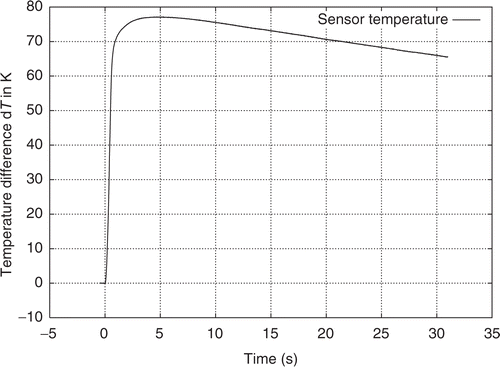
For the inverse problem aimed at finding the gas temperature G(t), t∈ [0, t^end], real measurements can be exploited as data (figure 3), where the simplified version of the arc test without additional textile material was performed for providing such data. The used constants based on the technological literature (for details see also 11 and 12) are specified by the following list: Here, χ_[a,b] is the characteristic function with respect to the interval [a,b]. The values β_Gas and β_Obj are products of dimensionless factors with the Stefan–Boltzmann constant. The domain is given by (12) and a maximal temperature G_max=8000K.

Figure 3. Calibration measurements of calorimeter temperature.

6.1. Determination without regularization

Since the calibration problem is a nonlinear inverse problem with smoothing forward operator F, local ill-posedness in the sense of [6, Definition 2] must be expected. For studying the ill-posedness effects occurring with equation (11) we first test a discretized version of the least-squares fitting (27) We suggest a Newton–CG algorithm for solving the problem (27). Let be an initial guess. Then the classical Gauss–Newton algorithm reads as , j=0,1, … , where the increment h_j denotes the solution of linear normal equation (28) Based on the knowledge of F′(G_j) and , we can use a CGLS-algorithm for solving (28) (e.g., [1, section 7.1]).

The Newton–CG algorithm is a modification of (28). The Newton step h_j is not calculated exactly, but approximated by the K-th CG iteration step h_j,K. The stopping index K=K(j) is chosen by an appropriate stopping criterion. For example we can choose K as smallest index which satisfies (29) for a constant 0<η <1 and a minimal tolerance TOLMIN. Choosing η not too small leads to a stabilization (regularization) of the algorithm 3. Additionally, we have to ensure, that . For this reason, a projection onto might be added in the algorithm.

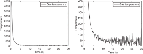
A solution G_ls of the extremal problem (27) for our data u_data is shown in figure 4. The peak of G_ls(t) in a neighborhood of t≈t_p=0.5s caused by the extreme energy of the electric arc seems to be approximated quite well. For times t after this peak, a temperature decay (first with a high and at the end with a low rate) occurs, but there we find strong oscillations of G_ls in the cooling phase, which are not physically interpretable and obviously express ill-posedness phenomena. Such oscillations cannot be accepted in the approximate solution of G for practical use, since forward computations of the arc test with real textile materials seem to be more sensitive to gas temperature changes in the final phase of cooling. This is due to the fact that the thermal conductivity of the isolation material is much lower than in the simplified test situation used for solving the inverse problem.

Figure 4. Gas temperature without regularization with zoom in the lower temperature interval.

6.2. A Tikhonov regularization approach

In order to overcome the drawback of ill-posedness, we should follow a regularization approach (cf. e.g., [1, 5]) for solving the operator equation (11) by a numerical procedure 15. Next, instead of (27) we use a discretized version of the second order standard Tikhonov method solving the extremal problem (30) with minimizer G_α. For existence and stability of such minimizers G_α for all α > 0 we refer, for example, 7. Note, that the term leads to a stronger penalization of the oscillations in the solution than the standard Tikhonov approach . Another reason for avoiding the latter term can be found in the structure of the solution. Penalization of the norm of the solution would flatten the peak in the gas temperature curve. Again we used a Newton–CG algorithm for solving the minimization problem (30). It can be done similarly to the least-squares fitting stated above. However, the normal equation (28) has to be replaced by the normal equation (31) of the Tikhonov functional (30), where the linear differential operator is defined as L G:=G′′ with domain .

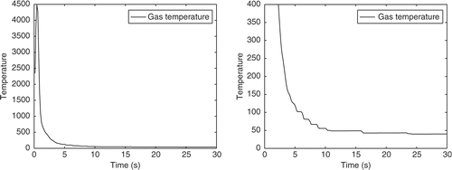
In our studies, the selection of the regularization parameter α > 0 was performed based on the quasi-optimality criterion (e.g., [4, p. 182]). It says that we choose the regularization parameter α as the minimum point of the functional for α∈(α_min,α _max). Given a sequence of parameters α_i=qⁱα₀ with α ₀=α_max and 0<q<1 the minimization can be done approximately by choosing α =α_i such that is minimal. The resulting quasi-optimal function G_α is shown in figure 5. Oscillations also occur in the cooling phase, but they are less and much smaller compared to the least-squares fitting. Note that the image function F(G_α) for the regularized solution is still a good approximation of the data function u_data. The obtained regularization parameter α and the relative error of the approximation can be found in table 1.

Figure 5. Gas temperature with second order Tikhonov regularization and zoom.

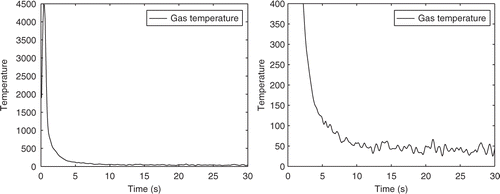
Table 1. Regularization parameters and relative data discrepancy values.

	α
Without regularization	–	1.1082 × 10^−4
Tikhonov regularization	2.2528 × 10^−6	9.7514 × 10^−4
Descriptive regularization	3.4337 × 10^−6	1.113 × 10^−3

We know the basic theoretical drawback (e.g., [1, Theorem 3.3]) of criteria for choosing the regularization parameter α that do not exploit the noise level δ satisfying , but unfortunately the rapidly increasing temperature of the calorimeter (figure 3) in connection with temperatures up to 5000 K near the arc and unknown inertia of the measurement system makes the prescription of a realistic δ required for the use of a discrepancy principle very problematic. On the other hand, the successful use of the quasi-optimality principle has been presented in very different practical applications in literature.

6.3. A descriptive regularization approach

As third approach, we use an ansatz of descriptive regularization. In detail, we add more a priori information about the qualitative behaviour of the gas temperature function, in particular the knowledge of monotonicity expressed by a more restricted domain During the burning time of the electric arc t∈ [0,t_p], we can assume a strictly growing function G(t). On the other hand, for sufficiently large t, here t≥ 2t_p, we have a monotone decay of the gas temperature. For the gap interval t∈(t_p, 2t_p) we do not impose additional requirements, but even for regularized solutions without monotonicity we have no oscillations in this time interval. Therefore, we define The regularized solution presented in figure 6 is obtained by solving a discretized version of (32) again based on a quasi-optimal choice of the regularization parameter α. The numerical realization was performed by a penalty method. The values of this approximate solution are not very different from the values G_α (t) for small t, but by construction the function suppresses oscillations nearly complete. Since the approximation error of u_data by (table 1) is nearly the same as for Tikhonov regularization, the solution seems to be the best approximation of the real gas temperature.

Figure 6. Gas temperature with descriptive regularization and zoom.

6.4. A numerical case study with synthetic data

To illustrate the results obtained, we finally present a case study based on synthetic data. We consider the function to be determined on the interval [0, t^end] with chosen t^end=30s again. Note that G*(t) has a similar structure as the gas temperature for the real data, but with a much lower peak at the beginning of the time interval. As data u_data we used a perturbation of the exact solution F(G*), where δ =10⁻⁴ and 10⁻³ denote the relative size of the added perturbations. In tables 2 and 3, we present the corresponding numerical results. It can be seen in table 2 that without regularization a relative error of 0.1% in the data leads to a relative error of about 15% in the solution, which shows the ill-posedness of the calibration problem. Using one of the two suggested regularization approaches for finding regularized solutions G_α we can stabilize the problem. However, the idea of descriptive regularization provides for both noise levels a better approximation of G*.

Table 2. Comparison of different solution approaches.

Without regularization		Tikhonov regularization		Descriptive regularization
δ		α		α
0	6.7512 × 10^−5	–	–	–	–
10^−4	0.0266	1.1973 × 10^−6	0.0056	9.6977 × 10^−7	0.0046
10^−3	0.1475	4.2391 × 10^−4	0.0152	3.4337 × 10^−4	0.0136

Table 3. Comparison of different parameter choice strategies.

	Morozov's discrepancy method		Quasi-optimality criterion
δ	α		α
10^−4	2.8243 × 10^−5	0.0112	1.1973 × 10^−6	0.0056
10^−3	1.668 ×^−3	0.0202	4.2391 ×^−4	0.0152

In table 2, the regularization parameter α is chosen by the quasi-optimality criterion. For a comparison, the final table 3 also presents the results obtained by using Morozov's discrepancy principle for Tikhonov regularization. Since we know the absolute noise level δ_abs for the synthetic data, we can apply the discrepancy principle which recommends to choose α =α (δ_abs) such that . We see that for both (relative) noise levels δ =10⁻⁴ and 10⁻³, the discrepancy principle provides a larger regularization parameter α and a worse approximation G_α of G* than the quasi-optimality criterion. This can be explained by the well-known overregularization effect of the discrepancy method. On the other hand, we see that the quasi-optimality criterion seems to be a good alternative for choosing the regularization parameter whenever the noise level δ is unknown.

7. Conclusions

•	For a computer-based simulation of electric fault arc tests, the determination of time-dependent gas temperature functions G=G(t) near the arc has to be realized. This function cannot be measured directly because of high temperatures and therefore it has to be calibrated by using indirect measurements based on temperatures u sufficiently far away from the arc.
•	In order to overcome the drawback of ill-posedness phenomena occurring in the corresponding nonlinear inverse problem of calibrating G, a regularization approach is required. Otherwise, strongly oscillating solutions are obtained which cannot be interpreted physically.
•	Second order Tikhonov regularization provides acceptable approximate solutions Gα of G for the calibration problem when the regularization parameter α > 0 is chosen by the quasi-optimality criterion.
•	The solution can further be stabilized and improved by using ideas of descriptive regularization, i.e., by exploiting the partial monotonicity of expected solutions.

References

- Engl, HW, Hanke, M, and Neubauer, A, 1996. Regularization of Inverse Problems. Dordrecht: Kluwer; 1996.
- Evans, C, 1998. Partial Differential Equations. Providence: AMS; 1998.
- Hanke, M, 1997. Regularizing properties of a truncated Newton–CG algorithm for nonlinear inverse problems, Numerical Functional Analysis and Optimization 18 (1997), pp. 971–993.
- Hansen, PC, 1998. Rank-Deficient and Discrete Ill-Posed Problems. Philadelphia: SIAM; 1998.
- Hofmann, B, 1986. Regularization for Applied Inverse and Ill-Posed Problems. Leipzig: Teubner; 1986.
- Hofmann, B, and Scherzer, O, 1994. Factors influencing the ill-posedness of nonlinear problems, Inverse Problems 10 (1994), pp. 1277–1297.
- Jakob, M, 1949. Heat Transfer. Vol. I. New York: John Wiley & Sons; 1949.
- Kunisch, K, and Ring, W, 1993. Regularization of nonlinear ill-posed problems with closed operators, Numerical Functional Analysis and Optimization 14 (3–4) (1993), pp. 389–404.
- International Social Security Association (ISSA), 2002. "Section Electricity–Gas–Long-Distance Heating–Water". In: Guideline for the selection of personal protective clothing when exposed to the thermal effects of an electric arc. 2002, c/o Berufsgenossenschaft der Feinmechanik und Elektrotechnik, Köln.
- Lady[zbreve]enskaja, OA, Solonnikov, VA, and Ural'ceva, NN, 1968. Linear and Quasilinear Equations of Parabolic Type. Providence, Rhode Island: American Mathematical Society; 1968.
- Schau, H, and Haase, J, 2002. Electric Fault Arc Calorimetric Analysis Based on ENV 50354:2000. Presented at Proceedings of the 6th International Conference on Live Maintentance (ICOLIM 2002).
- Steinhorst, P, 2003. "Simulation of the nonstationary heat transfer through heat protecting textiles (in German)". Chemnitz: Chemnitz University of Technology; 2003, Diploma thesis, Faculty of Mathematics.
- Steinhorst, P, Hofmann, B, Meyer, A, and Weinelt, W, 2005. Gas temperature identification for the simulation of electric fault arc tests. Presented at 5th International Conference on Inverse Problems in Engineering: Theory and Practice. Cambridge, 11–15 July, 2005, In: D. Lesnic (Ed.).
- Torvi, DA, and Dale, JD, 1999. Heat transfer in thin fibrous materials under high heat flux, Fire Technology 35 (3) (1999), pp. 210–231.
- Vogel, CR, 2002. Computational Methods for Inverse Problems. SIAM: Philadelphia; 2002.
- Zeidler, E, 1985. Nonlinear Functional Analysis and its Applications I–Fixed-Point Theorems. New York: Springer; 1985.