Experimental validation of an extended Kalman smoothing technique for solving nonlinear inverse heat conduction problems

Abstract

A new approach combining the use of the Kalman filter with an extended version of a smoothing technique and introducing the use of future time measurements is developed in order to improve the solution of a nonlinear Inverse Heat Conduction Problem (IHCP). The behaviour of the proposed algorithm is analysed in presence of a real set of experimental noisy temperature measurements. Estimation results are validated by using a space marching technique proposed by Raynaud and Bransier whose performance is already known for the solution of the one-dimensional nonlinear IHCP. The influence of the number of future time data on the accuracy and the stability of the solution is analyzed according to the inverse time step, the location of the measurement sensor, and the standard deviation of the modeling error. Effects of the standard deviation associated with the measurement errors and the second boundary condition on the inverse solution are also investigated.

Keywords:

• Kalman smoothing technique
• Nonlinear inverse problem
• Future time measurements
• Experimental study.

Keywords:

• 2000 Mathematics Subject Classifications: 80A20
• 80-05
• 80A23
• 93B18
• 93C10
• 60G15
• 62M20

Nomenclature

C:	=	volumetric heat capacity
D:	=	diameter of the cylinder
e:	=	thickness of the cylinder
H:	=	observation matrix
I:	=	identity matrix
K:	=	gain matrix
n:	=	total number of time steps
nf:	=	number of future measurements
P:	=	covariance matrix of estimation error
q:	=	heat flux density
Q:	=	covariance matrix of model error
R:	=	covariance matrix of measurement errors
t:	=	time
T:	=	temperature
T0:	=	initial temperature
x:	=	state vector
y:	=	vector of measurements
y:	=	measurement
z:	=	spatial coordinate

Greek Symbols

α:	=	thermal diffusivity
Δt:	=	inverse time step
Δt*:	=	dimensionless inverse time step ()
λ:	=	thermal conductivity
σm:	=	standard deviation of measurement errors
σq:	=	standard deviation of the modeling error

Subscripts and Superscripts

⁁:	=	estimation sign
-:	=	prediction sign
1, 2, 3, 4:	=	refer to the four measurement sensors
k:	=	number of time steps
m:	=	refers to measurement
tr:	=	transposition operator

1. Introduction

Due to the diffusive nature of the heat conduction, surface temperature changes are damped and lagged in the interior of the solid. Hence small inaccuracies in the measured interior temperatures can cause large oscillations in the estimated surface conditions which can show a time lag dependent on the measurement location. Based on the fact that the response of a temperature sensor placed at a distance below a heated surface can continue to rise even after the applied surface heat flux returns to zero, Beck was the first to recognize that a precise estimation of surface conditions requires the use of temperatures measured at times ulterior to the time of estimation and known as future time measurements 1.

The use of future temperatures was first applied by Beck 2 to the Duhamel's theorem solution of the IHCP, then combined for the first time with difference methods by Beck and Wolf 3. In its original version that represents a reference for inverse methods in heat transfer, the function specification method proposed by Beck 4 uses future time temperatures in a procedure based on the minimization of the least squares error between computed and measured temperatures. This method underwent different improvements. It was combined by Osman et al. 5 with a regularization technique, then modified by Blanc et al. 6 using a time-variable number of future temperatures. Raynaud and Bransier have also introduced 7 future time temperatures in the analysis of the IHCP using a space-marching finite-difference procedure which is as precise as the Beck's method as shown in 8.

In this study, we introduce the use of future time measurements in a new approach combining the Kalman filter 9 with an extended version of a smoothing technique. The proposed algorithm 10 is developed in order to improve the solution of a nonlinear transient one-dimensional IHCP involving reconstruction of the heat flux density and the temperature at the surface of a cylindrical heat conducting solid. The aim of this work is to analyse the behaviour of the extended Kalman smoothing technique in presence of a real set of experimental noisy temperature measurements.

The influence of the number of future time data on the accuracy and the stability of the solution is studied according to the location of the measurement sensor, the standard deviation associated with the modeling error, and the inverse time step. Estimation results are validated with the solution of the space marching technique proposed by Raynaud and Bransier 7, whose performance is already known for the solution of one-dimensional nonlinear IHCP 8. Effects of the standard deviation associated with the measurement errors and the second boundary condition of the problem obtained by using measured temperatures are also investigated.

2. Problem description

2.1. Experimental set-up

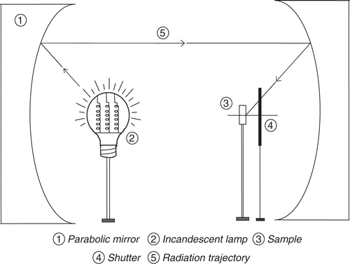
The surface of a cylindrical sample in stainless steel of diameter D = 14 mm and thickness e = 15 mm is submitted to a radiative heat flux coming from a reflection furnace built in the center of heat transfer at INSA (Lyon–France) and which allows to apply a uniformly distributed surface heat flux density (figure 1). This reflection furnace is composed of two parabolic mirrors made of crystal and having each a diameter of 1.5 m and an opening angle of 120°. The surface heat flux comes from an incandescent lamp whose radiation is concentrated toward the sample by one or several reflections on the two mirrors.

Figure 1. Sketch of the experimental set-up.

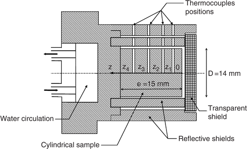
In order to minimize lateral heat transfer, two reflective shields in stainless steel are placed around the cylinder while letting an air thickness of 1 mm. Air of the same thickness also separates the two shields (figure 2). A transparent shield in glass of diameter 25 mm and thickness 4 mm is placed against the surface of the sample to avoid convective heat transfer. This surface is covered by a black painting (total emissivity 0.98) in order to increase absorption of the radiation coming from the furnace. The back side of the cylinder is cooled by a water circulation.

Figure 2. Description of the cylindrical sample.

The thermal diffusivity α and the volumetric heat capacity C of stainless steel are determined experimentally, as described in 11, for temperatures varying between 256 K and 417 K. In this range of temperatures, variation of thermal diffusivity is negligible. Its assumed constant value is α = 3.87 × 10⁻⁶ m² s⁻¹.

Variation of volumetric heat capacity with temperature is given by,

The thermal conductivity is calculated using the following relation:

Four thermocouples (type K, wire diameter: 0.1 mm) are spot welded inside the sample on its axis at known positions (within ±0.05 mm): z₁ = 2.1 mm; z₂ = 4.1 mm; z₃ = 8.1 mm and z₄ = 12.1 mm (figure 2). Temperature measurements are recorded by a Keithley device (model 575) with a maximum rate of 20 readings per second.

2.2. Mathematical model

The problem under study is described by the one-dimensional nonlinear heat conduction equation for homogeneous and isotropic material: (1) subject to the following initial and boundary conditions: (2) (3) (4) where T is the temperature, z is the spatial coordinate, t is the time, q is the heat flux density and T₀ is the initial temperature assumed to be uniform.

Ignoring the boundary condition at z = e (figure 2), we limit our survey to the region between z = 0 and z = z₄ where the transient temperature measurements at z₄ denoted as y⁴(t) are assumed to be the second boundary condition of the model [equation (4)]. The boundary condition at z = 0 [equation (3)], which is the heat flux density, is unknown and will be estimated as a function of time with the inverse method. The solution of the considered inverse problem requires the use of transient temperature measurements taken in z = z_m (m = 1, 2, 3) which leads to additional conditions written as, (5)

These measurements are used in the inverse technique in order to estimate simultaneously with the surface heat flux density q(t) the time variation of the surface temperature T(0, t).

3. The extended Kalman smoothing technique

The Kalman filter is a stochastic recursive estimator which provides a solution to linear filtering problems 12. An extended version of the Kalman filter was proposed and applied by Daouas and Radhouani in 13 to solve a nonlinear inverse heat conduction problem. The same authors proposed in 11 a guide for a suitable choice of the filter covariance matrices in order to obtain a good reconstruction of surface conditions. This extended version provides a solution that remains stable in presence of real noisy measurements but that is time-lagged compared to the exact solution.

The proposed algorithm 10 introduces the use of future time measurements in order to avoid the lag in the response and obtain a symmetrical solution. This algorithm combines the extended Kalman filter with a new version of the fixed interval smoothing technique capable of handling the nonlinear inverse heat conduction problem under study.

Nonlinear equations of the problem are modified by linearization about some reference state vector. Then, the original formulation of the smoothing technique, referred to as the RTS (Rauch Tung Striebel) algorithm 14, is applied to the linearized equations. Owing to this new approach, the state at time t_k is estimated using n_f observations ulterior to the estimation time, where n_f is the fixed number of future measurements. This allows introducing the use of future measurements in the Kalman filter technique.

In case of nonlinear systems, the state vector x and the measurements vector y are, respectively, represented by the following relations: (6) (7) where and are non-linear vectors, V_k and W_k are noise vectors, associated, respectively, to the model and the measurements, that are white and Gaussian and have zero mean.

The initial state x₀ is also considered a Gaussian random variable whose covariance matrix is denoted as P₀.

The formulation of the Kalman filter is based on the determination of the minimum variance estimate that minimizes the mean square estimation error , where E[.] is the “expected value operator”. It is shown in 9 that the minimum of this mean square error is given by the mean of the state vector x_k conditioned on the available observations Y, written as: . In the Gaussian case, this enables us to write out an explicit expression for the optimal estimate in recursive form.

This formulation applied to the linearized equations of the problem leads to the extended Kalman filter algorithm which takes place in a recursive manner in two stages 15:

•

the prediction at tk+1 based on the model and the observations until tk, (8) and the covariance matrix associated with this prediction, (9)

•

the correction of the prediction using the new information given by the observation at tk+1, (10) and the covariance matrix associated with this estimation, (11) where and denote predictions, and Pk denote estimations and Fk and Hk+1 are matrices written as, Q is the covariance matrix of the model error, K is the Kalman gain given by, (12) I is the identity matrix, H is the observation matrix and R is the covariance matrix of measurement noise.

We adopt the same linearization used with the extended Kalman filter in 9, whose reference vector is updated with the filter estimates getting at each time the value of the last available estimation. So the fixed interval smoothing technique leads to the following recursive relation 10: (13) where (14) represents the state estimation at time t_k using n_f = (n − k) future measurements, where n is the total number of time steps.

The computational procedure summarized in figure 3, takes place in a forward recursive sweep followed by a backward sweep which provides a fixed-lag smoothing by first filtering up to the current measurement at time t_k using the extended Kalman filter algorithm [equations (8–12)] and then sweeping back n_f = (n − k) steps with the recursive equation of RTS algorithm [equations (13a and b)]. The old filter estimate is so updated to yield an improved smoothed estimate which uses further n_f future measurement data. At each new time step, a new prediction and a new estimation of the extended Kalman filter are saved, whereas oldest ones are discarded since we need only the n_f most recent filter results for the backward sweep. So, with each new measurement, we have like a sliding window of data by moving one step forward and n_f steps back.

Figure 3. Procedure for fixed-interval smoothing.

Since we are interested in estimating the time variation of the surface heat flux density in addition to the correction of the process state x_k (composed by nodal temperatures within the sample and on the surface), we apply the above estimation algorithm using an augmented state vector X_k defined in 16 as X_k = [x_k, q_k]^tr, where q_k is considered a further state variable appended to the original ones and assumed to be piecewise constant. This approximation leads to estimate a succession in time of constant parameters.

4. Results and discussions

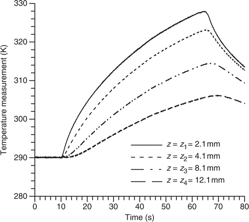
Temperatures represented in figure 4 are recorded from the four thermocouples for a lamp heat power of 1000 W, that is 40 W cm⁻². At t = 0, temperatures measured from the four sensors (before the heating starts) are, respectively: T(z₁, 0) = 290.03 K, T(z₂, 0) = 290.00 K, T(z₃, 0) = 290.00 K, T(z₄, 0) = 289.96 K. The average value of the four above temperatures (T₀ = 289.99 K) is taken as the initial temperature of the cylinder considered uniform. This approximation is taken into account by the Kalman filter which assumes the initial state to be a Gaussian random variable, and enables us to associate an error covariance matrix to this initial estimation.

Figure 4. Recorded temperatures from the four thermocouples.

Using the shutter (figure 1), a square heat flux density is applied on the surface of the cylinder during 58 s. One of the main disadvantages of this concentration system is the important optical losses due notably to reflection on the mirrors. The aim of this work is to estimate the fraction of the source radiation really concentrated toward the sample. Time variations of this surface heat flux density and the surface temperature are determined using measurements provided by one of the three thermocouples placed in z₁, z₂ or z₃ as shown in figure 2. The other two measurements will be used for the comparison with calculated temperatures. Transient temperature measurements taken at z₄ are regarded as being the second boundary condition of the problem. In this one-sensor case, the covariance matrix R of the measurement noise is reduced to a scalar quantity equal to the variance . The standard deviation relative to the measurement noise is taken as σ_m = 0.05 K, which is an average value of the standard deviations that we estimated for each of the sensors before the heating starts.

Inversion results of the Kalman filter and the Kalman smoother are validated by using the Raynaud and Bransier inverse method. The accuracy of estimated surface conditions is also analysed by superposing computed (calculated with the estimated heat flux density) and measured temperatures and by calculating the relative error between these two temperatures defined as 17, (15) where y_i is the measured temperature, T_i is the computed temperature at the sensor location at time corresponding to the i-th measurement and M = m * n (m is the number of sensors used for comparison equal to 3 in this study and n is the number of temperature recordings per thermocouple during the experiment).

An explicit finite-difference scheme is used for the prediction calculations. This scheme is adopted, despite of its stability constraint 18, in order to obtain a simple representation of the state equation which can easily correspond to the prediction equation of the extended Kalman filter [equation (8)].

Time variations of surface heat flux density and surface temperature are estimated using different positions of the measurement sensor providing information needed for the inversion. The inverse time step (time interval separating two successive measurements) is taken as Δt = 0.1 s. The standard deviation of the modeling error which is a stabilizing parameter in the Kalman filter algorithm 1113, is assumed to be constant and is taken as σ_q = 100 W m⁻². This parameter is associated with the diagonal covariance matrix Q whose only element different from zero is the variance so as to compensate the model mismatch caused by the unknown heat flux approximation with a piecewise constant function.

According to figures 5a and 6a, one can note that the Kalman filter estimates show a time-lag when superposed to the Raynaud method solution. This validation solution is obtained in all cases by using the first sensor located at z₁ and by applying a prefiltering of the input data in order to reduce important oscillations that appeared notably in the estimated surface heat flux. The time lag of the Kalman filter solution increases as the distance between the sensor and the active surface (subject to the heat flux) is larger. In this case, the solution, notably the heat flux density, becomes less stable.

Figure 5. Influence of the measurement location on the surface heat flux density estimations (Δt = 0.1 s, σ_q = 100 W m⁻²): (a) without smoothing; (b) with smoothing.

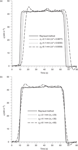
Figure 6. Influence of the measurement location on the surface temperature estimations (Δt = 0.1 s, σ_q = 100 W m⁻²). (a) Without smoothing; (b) with smoothing.

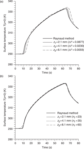
The Kalman smoother allows obtaining a symmetrical and more stable solution whose superposition with the validation method estimation is improved, by using a number of future measurements dependent on the measurement location. As shown in figures 5b and 6b, a farther sensor from the surface requires a larger number n_f of future time measurements. These results are also illustrated by calculating values of the global relative error (ERR) and the maximum relative error shown in table 1.

Table 1. Influence of the measurement location on the accuracy of the inverse solutions with or without smoothing

	ERR (%)		Maximum relative error (%)
Measurement location zm	No smoothing	Smoothing	No smoothing	Smoothing
z1	0.188	0.034	1	0.248
z2	0.323	0.038	1.53	0.356
z3	0.553	0.084	2.42	0.591

An optimal value of n_f is obtained by increasing it progressively while observing the solution behaviour. At a first time, the solution is only shifted on the left. Then oscillations are reduced and a slight shift on the left is also noted. We continue increasing the value of n_f until it provides no further improvement of the estimates. This point is detailed in 10.

Figure 7a shows the behaviour of the Kalman filter for three different values of the standard deviation σ_q. Decreasing this parameter, the response of the filter becomes slower leading to an increase in the solution time lag. On the other hand, one can note a reduction of oscillations which means that the solution becomes less sensitive to measurement errors. So the choice of σ_q must satisfy a compromise between stability and precision as explained in 13. In such real estimation where no exact values can be compared, the choice of this stabilizing parameter is guided by the observation of the solution behavior. Based on the results of the previous work 13, where a numerical simulation was carried out, a dimensionless value σ_q/q_max ≈ 0.025 leads to a minimum bias which involves both estimation errors of the model and perturbations affecting the measurements. This value may vary with the measurement sensor location and with the level of the measurement noise. It is used first as an initial estimation of the standard deviation. Then it is adjusted according to the solution behaviour as explained earlier, where trial and error is typically used.

Figure 7. Influence of the modeling error standard deviation on the estimation of the surface heat flux density (z₁ = 2.1 mm, Δt = 0.1 s, Δt* = 0.0877): (a) with the Kalman filter; (b) with the Kalman smoother.

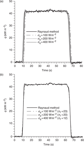
The use of the extended Kalman filter smoothing technique with an optimal number of future time data provides a symmetrical and more stable solution that is in good agreement with the heat flux density estimated with the Raynaud method (figure 7b). The number of future data (listed for each case in figure 7b) depends on the value of σ_q. It increases as σ_q decreases. Choosing the n_f value according to the σ_q value, we obtain nearly the same global relative error ERR (table 2) showing a very good superposition between calculated and measured temperatures.

Table 2. Influence of the modeling error standard deviation on the accuracy of the inverse solutions with or without smoothing

	ERR (%)		Maximum relative error (%)
Standard deviation σq (W m^−^2)	No smoothing	Smoothing	No smoothing	Smoothing
100	0.188	0.034	1	0.248
200	0.141	0.035	0.77	0.201
400	0.109	0.032	0.61	0.133

One of the main difficulties of the IHCP is the increase of the solution sensitivity to measurement errors when using small inverse time steps. For one dimensional inverse problems, we can check the feasibility of the surface conditions estimation by calculating a dimensionless time step characteristic of the inverse problem, given in 19 by, (16)

Raynaud stated in 19 that inverse resolution is feasible when Δt* > 10⁻³. Otherwise, it becomes very sensitive to experimental errors affecting measurements. On the other hand, choosing a large value of the inverse time step doesn’t allow to represent abrupt variations of the estimated function and leads to a solution that is not precise. As shown in figure 8a, the behaviour of the Kalman filter using different inverse time steps confirms the above mentioned fact. In the present study, the dimensionless time step Δt* is calculated using the assumed constant value of the thermal diffusivity. In case α depends on temperature, Δt* is defined in 7 by using α (T₀).

Figure 8. Influence of the inverse time step on the surface heat flux density estimations. (σ_q = 100 W m⁻², z₁ = 2.1 mm): (a) with the Kalman filter; (b) with the Kalman smoother.

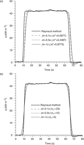
By introducing the use of future time data in the inverse procedure, we obtain a more precise and more stable estimation which is symmetrical according to the Raynaud method solution (figure 8b). The results show that a larger number of future time data is required when using smaller inverse time steps. Figure 8b shows that n_f = 5 is satisfactory for Δt = 1s, whereas a larger number (n_f = 23) is needed for Δt = 0.1 s.

Estimation results are validated by calculating the associated values of the relative error between measurements and temperatures computed with the estimated heat flux density (table 3).

Table 3. Influence of the inverse time step on the accuracy of the inverse solutions with or without smoothing

	ERR (%)		Maximum relative error (%)
Inverse time step Δt (s)	No smoothing	Smoothing	No smoothing	Smoothing
0.1	0.188	0.034	1	0.248
0.5	0.272	0.041	1.30	0.317
1	0.324	0.064	1.48	0.343

The Kalman filter formulation based on a statistical approach allows a description of the stochastic structure of experimental measurements using a vector modelization of the measurement noise. Information about this noise is required in the Kalman filter algorithm by introducing the associated covariance matrix R. In the present study, we use real noisy measurements whose noise standard deviation is estimated to σ_m = 0.05 K. The behaviour of the Kalman filter solution is analysed when experimental data are assumed to be noise-free (i.e. σ_m = 0 K). In this case, the solution shows important oscillations (figure 9) because measurement errors are underestimated and noise is not sufficiently filtered. On the other hand, this solution is more accurate (symmetrical compared with the Raynaud method solution) because the filter grants more confidence to the measurements and less confidence to the model predictions. Using a larger value of the noise standard deviation (σ_m = 0.5 K), the transient performance of the Kalman filter is slower (figure 9). Indeed, the Kalman gain K decreases as the covariance matrix R increases. In this case where the measurement errors are overestimated, the noise is filtered out and the solution is very smooth.

Figure 9. Influence of the standard deviation associated with the measurement noise on the Kalman filter behavior (σ_q = 100 W m⁻², z₁ = 2.1 mm, Δt = 0.1 s, Δt* = 0.0877).

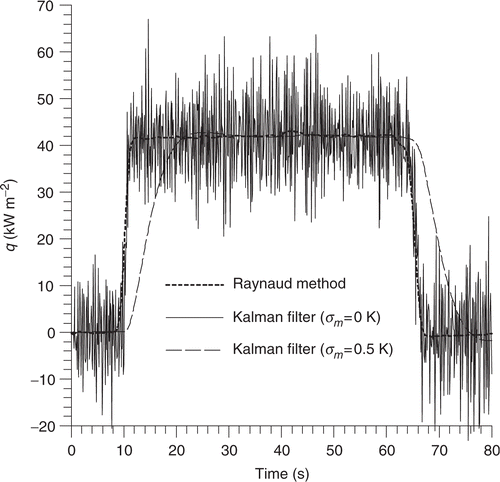
When the noise standard deviation underestimates the real value, estimation error provided by the filter is smaller than the actual error. A noise standard deviation which overestimates the real value entails an estimation error larger than the actual one. This fact is illustrated in table 4 for heat flux density estimated at t = 40 s.

Table 4. Effect of the SD associated with the measurement noise on the estimation error provided by the Kalman filter

σm (K)	q (kW m^−^2)	Estimation error (kW m^−^2)
0	47.406	±0.173
0.05	41.983	±0.380
0.5	41.898	±0.667
1	42.334	±0.803

In the case where σ_m = 0.5 K, the solution shows an important time lag (ERR = 0.554%) and requires a large number of future time measurements to be symmetrized. Applying the Kalman smoother with n_f = 70, we obtain a symmetrical solution which provides a better superposition between measured and computed temperatures (ERR = 0.084%). However, this solution is very smooth and doesn’t represent abrupt variations of the estimated heat flux density. When measurements are assumed to be noise-free, a number of future measurements n_f = 5 provides a slightly improved estimation of the surface heat flux density. Indeed, the global relative error between measured and calculated temperatures decreases from ERR = 0.0468% to ERR = 0.0320%. Increasing n_f has no further influence on the solution. In this case, the Kalman smoother estimation still contains important oscillations.

The transient temperature measurements provided by the fourth thermocouple placed at z₄ = 12.1 mm (figure 2) are taken as the second boundary condition of the problem. The effect of this boundary condition on the inverse solution is studied by superposing to these measurements an additional Gaussian random error of different values of standard deviation σ, and by calculating for each standard deviation the relative error between measured and computed temperatures. Estimation of the heat flux density is made with the following parameters: Δt = 0.1 s, z₁ = 2.1 mm, σ_m = 0.05 K, σ_q = 200 W m⁻², n_f = 20. As shown in table 5, there is no considerable increase in the relative error even when the standard deviation reaches the value σ = 2 K, which is large compared with the level of noise corresponding to the present experimental set-up.

Table 5. Effect of the second boundary condition on the Kalman smoother solution

σ (K)	ERR (%)	Maximum relative error (%)
0	0.035	0.201
0.1	0.036	0.201
0.5	0.037	0.201
1	0.039	0.202
2	0.044	0.202

5. Conclusions

An experimental study was carried out in order to analyse the behaviour of a new approach, combining the use of the Kalman filter with a smoothing technique, when applied with real measurements recorded from an experimental set-up.

The proposed algorithm, developed to handle nonlinear inverse problems, provides a better estimation of time-varying surface conditions, involving heat flux density and temperature, whose time lag and sensitivity to measurement errors are reduced. Introducing the use of an optimal number of future time measurements, the improvement in the estimation due to the Kalman smoother is proved by a good superposition with the solution of the space marching method taken as the validation inverse method. The Kalman smoother inverse solution is also validated by the good superposition between computed and measured temperatures.

The effect of the number of future time data on the accuracy and the stability of the solution have been investigated. The results show that the number of future temperature measurements needed to obtain a symmetrical solution increases as the standard deviation associated with the modeling error decreases. A larger number of future time data is also required when using smaller inverse time steps or when the measurement sensor is placed farther from the surface on which the heat flux is applied. The effect of the measurement noise estimation was analysed by associating standard deviations (required in the Kalman algorithm) which underestimate and overestimate the real value. The obtained results showed that a statistical description of measurement noise that fits the real experimental conditions of the problem is needed in order to get symmetrical and stable solutions. Investigation of the influence of the second boundary condition showed that it has no considerable effect on the inverse solution for the range of noise standard deviation obtained with the studied experimental set-up. A suitable choice of the parameters of the problem guided by the smoother behaviour provided a good estimation of the surface condition which is symmetrized with the use of an optimal number of future time measurements.

Compared to other inverse techniques involving the Raynaud method, the Kalman algorithm presents some interesting features. Its formulation based on a statistical approach permits one to describe the random structure of the experimental measurements and to take into account the variance of the initial estimation, and gives information concerning the quality of estimation. This algorithm provides estimates of the whole state vector by optimally smoothing errors affecting both the initial temperature distribution and the surface condition. According to the obtained results, the proposed algorithm is not significantly affected by measurement errors. Indeed, its application with real noisy measurements does not disrupt the stability of the estimation process.

On the other hand, when applying the Raynaud method, prefiltering of the input data was required in order to reduce oscillations that appeared in the solution. This simple and efficient technique shows good performance when applied to nonlinear one-dimensional inverse problems, but does not readily extend to multiple sensors and multidimensional cases.

The troublesome feature about the proposed Kalman smoother technique is the rapid increase of computational time and memory when we want to improve the spatial accuracy. This difficulty is due to the enormous increase of the algorithm vectors and matrices and to the stability condition of the explicit scheme that requires the use of much smaller time steps. So a great deal of computer memory and speed should be considered.

References

- Minkowycz, WJ, Sparrow, EM, Schneider, GE, and Pletcher, RH, 1988. Handbook of Numerical Heat Transfer. New York: Wiley Interscience; 1988.
- Beck, JV, 1968. Surface heat flux determination using an integral method, Nuclear Engineering Design 7 (1968), pp. 170–178.
- Beck, JV, and Wolf, H, 1965. "The non linear inverse heat conduction problem". In: ASME Paper, 65-HT-40. 1965.
- Beck, JV, 1970. Non linear estimation applied to the non-linear inverse heat conduction problem, International Journal of Heat and Mass Transfer 13 (1970), pp. 703–716.
- Osman, AM, Dowding, KJ, and Beck, JV, 1997. Numerical solution of the general two-dimensional inverse heat conduction problem (IHCP), Transactions of the ASME 119 (1997), pp. 38–44.
- Blanc, G, Beck, JV, and Raynaud, M, 1997. Solution of the inverse heat conduction problem with a time-variable number of future temperatures, Numerical Heat Transfer (B) 32 (1997), pp. 437–451.
- Raynaud, M, and Bransier, J, 1986. A new finite difference method for the non-linear inverse heat conduction problem, Numerical Heat Transfer (B) 9 (1986), pp. 27–42.
- Raynaud, M, and Beck, JV, 1988. Methodology for comparison of inverse heat conduction methods, Journal of Heat Transfer 110 (1988), pp. 30–37.
- Brown, RG, and Hwang, PYC, 1992. Introduction to Random Signals and Applied Kalman Filtering. New York: John Wiley and Sons; 1992.
- Daouas, N, and Radhouani, M-S, 2004. A new approach of the Kalman filter using future temperature measurements for nonlinear inverse heat conduction problems, Numerical Heat Transfer (B) 45 (2004), pp. 565–585.
- Daouas, N, and Radhouani, M-S, 2002. Analyse de la qualité de restitution d’un flux de chaleur surfacique provenant d’un four estimé à l’aide d’une technique inverse statistique, Revue. Entropie 242 (2002), pp. 57–63.
- De Shutter, J, De Geeter, J, Lefebre, T, and Bruyninckx, H, 1999. Kalman filters: a tutorial, Journal A [J.A.] 40 (4) (1999), pp. 52–59.
- Daouas, N, and Radhouani, M-S, 2000. Version étendue du filtre de Kalman discret appliquée à un problème inverse de conduction de chaleur non linéaire, International Journal of Thermal Sciences 39 (2000), pp. 191–212.
- Rauch, HE, Tung, F, and Striebel, CT, 1965. Maximum likelihood estimates of linear dynamic systems, AIAA Journal 3 (1965), pp. 1445–1460.
- Labarrere, M, Krief, JP, and Gimonet, B, 1982. Le Filtrage et ses Applications. 1982, Cepadues Editions.
- Scarpa, F, and Milano, G, 1995. Kalman smoothing technique applied to the inverse heat conduction problem, Numerical Heat Transfer (B) 28 (1995), pp. 79–96.
- Huang, C-H, Yuan, I-C, and Ay, H, 2003. A three dimensional inverse problem in imaging the local heat transfer coefficients for plate finned-tube heat exchangers, International Journal of Heat and Mass Transfer 46 (2003), pp. 3629–3638.
- Patankar, SV, 1980. Numerical Heat Transfer and Fluid Flow. New York: Hemisphere/Mc Graw-Hill; 1980.
- Raynaud, M, 1995. "Applications des méthodes de conduction inverse à la mesure des températures et flux surfaciques transitoires". In: Proceedings of ≪50° Congresso, Associazione Termotecnica Italiana (ATI)≫. Saint-Vincent. 1995. pp. 345–356.