Initial temperature reconstruction for nonlinear heat equation: application to a coupled radiative–conductive heat transfer problem

Abstract

In a cooling process described by a nonlinear heat equation, we are interested to recover the initial temperature from the temperature measurements that are available on a part of the boundary for some time. Up to now, even for the linear heat equation, this problem usually has been studied as a nonlinear ill-posed operator equation, and regularization methods involving Fréchet derivatives have been applied. We propose a fast derivative-free iterative method. Numerical results are presented for the glass cooling process where the nonlinearity appears due to radiation.

Keywords:

• Initial temperature reconstruction
• Radiative–conductive heat transfer
• Derivative-free iterative method
• Inverse problem
• Regularization

2000 Mathematics Subject Classifications:

• 80A23
• 65M32

1. Introduction

In many cooling processes (e.g., in glass production 1,2, polymer processing 3,4), it is important to avoid large temperature differences inside the material. However, the information about the inside temperature is frequently unavailable because its measurement is extremely difficult and sometimes even impossible. On the other hand, the boundary temperature measurements can be made much easier. Thus, we are faced with the problem of reconstructing the temperature inside the material from the temperature on its boundary.

We will consider a cooling process that is modeled by the heat equation with a source term nonlinearly dependent on the temperature. Since the temperature in the body is uniquely determined by the initial temperature, it is sufficient to reconstruct only the initial temperature.

Previously, reconstruction of the initial temperature from boundary measurements was considered only for the linear heat equation 3–5 with source terms independent of the temperature. In 3,4, the problem was formulated as a constrained minimization problem. Minimization was performed by the conjugate gradient method, resulting in the necessity to compute Fréchet derivatives. Extension of this idea to a nonlinear heat equation results in both theoretical and computational difficulties. In 5, the initial temperature was considered as the solution to some operator equation. Although the original equation was nonlinear, using a proper affine decomposition 6, it was reduced to a linear equation. We propose to use this reduction in constructing an iterative method for our problem. This method does not involve computation of derivatives. Each iteration consists of solving an ill-posed linear equation with a fixed operator. Due to ill-posedness, this equation needs to be regularized. The proposed method does not depend on the concrete type of the nonlinear source term and can be easily applied for multidimensional problems.

The structure of the article is as follows. In section 2, we present a 1D model for the cooling of a glass plate. This model consists of a nonlinear heat equation due to heat radiation effects. We use this model as a prototype for a general nonlinear heat equation. We also formulate the nonlinear operator equation for the initial temperature. The proposed iterative method and regularization issues are presented in section 3. Numerical results are presented in section 4. Finally, we make conclusions and give an outlook in section 5.

2. Problem formulation

2.1. Mathematical model for the cooling of a glass plate

Let us first present the mathematical model for the cooling of a hot glass plate. In this process, one usually neglects variation of the plate temperature along its height and width and considers spatial dependence of the temperature only on the thickness 3,7–9. Thus, the temperature T(z, t) is a function of the thickness z∈ [0,l] and time t∈ [0,t_f].

Without internal heat sources or sinks, the temperature T satisfies the well-known heat equation where c_m, ρ_m, k_h are specific heat, density and thermal conductivity of the material that are assumed to be constant. For the processes involving high temperatures, the heat transfer by radiation needs to be taken into account. An introduction to this subject can be found, e.g. in 10. Next, we give the features that are essential for the glass cooling 8,9,11.

The radiation field is described by the radiative intensity that is, in general, a function of position r, time t, direction s, and frequency ν. In analogy to the temperature, we may assume that the radiative intensity depends actually only on the thickness z and direction coordinate μ∈ [-1,1] along the thickness. The governing equation for I, the so-called radiative transfer equation, depends on the radiative properties of the material. The assumption of an absorbing, emitting, and nonscattering medium is frequently justified for glass. In this case, the radiative transfer equation has the following form: (1) where κ (ν) is the absorption coefficient for the glass,1 and P(T,ν) is Planck's function defined by where are Planck's and Boltzmann's constants, c₀ is the speed of light in vacuum, and n_g is the refractive index of the material.

Equation (1) needs to be equipped with boundary conditions. We consider the so-called black surface boundary conditions (2) where T_a is the ambient temperature.

The frequency domain is divided into two regions: the opaque region [0,ν ₁) where κ (ν) =∞, and the semitransparent region [ν ₁,∞) where κ (ν) <∞. The electromagnetic waves with the frequencies from the semitransparent region are responsible for the radiative heat transfer inside the material, whereas the waves from the opaque region are involved in the radiative heat transfer on the boundary.

Thus, including the radiation effects, the heat equation has the following form: (3) with the boundary conditions (4) and the initial condition (5) The boundary conditions (4) are derived, e.g., in 8. In (4), we have neglected the convective heat exchange along the boundary. This is justified for large temperatures when the heat exchange by radiation is dominant (see, e.g., 11).

The well-posedness of the coupled system (1–5) has been rigorously shown for some particular cases, see 12,13 and the references therein. One possible numerical method for its solution can be found in, e.g., 14. We briefly describe it here. First of all, we assume that the semitransparent frequency region [ν ₁,∞) is divided into M spectral bands so that Then one considers the integrated spectral characteristics and the integral reduces to the sum involving P_k and I_k. For approximating the integral one uses the so-called Discrete Ordinates method (S_P-approximation) [10, p. 541], which consists in choosing numbers such that Thus, the whole source term in (3) is approximated by where the functions are determined by the equations with the boundary conditions These equations are approximately solved by some finite difference approximation of the derivative . Finally, equation (3) is also approximated by a finite difference scheme.

2.2. Inverse problem for a general heat equation with a nonlinear source term

Let us write (3–5) in the following scaled and compact form (6) where n(z_b)=-1 for z_b = 0, and n(z_b)=1 for z_b = l. If the initial temperature was known, we would be able to obtain the temperature inside the material for the later time. However the measurements of the temperature inside a hot body are extremely difficult, and thus the initial data u is unknown. Fortunately, we have boundary temperature measurements at hand. The boundary temperature is often known not on the whole boundary, but only on some part of it. Since in 1D the boundary consists only of two points {0,l }, we assume that the temperature D(t) is known at the point z_b = 0 in the time interval [0,t_f]. Let denote a nonlinear operator that maps the initial temperature to the boundary temperature. Then, the initial temperature u satisfies the nonlinear operator equation (7) In the case when the source and flux terms in (6) do not depend on the temperature, the operator equation for the initial temperature was studied in 5. Since we will use this equation in the iterative method for the solution of (7), we state it for a later reference. For this purpose, examine the linear heat equation Denote the corresponding boundary temperature at z_b = 0 as d(t):=T(z_b,t) for t∈ [0,t_f]. Consider an operator that maps functions , , to the function d(t), where and are admissible function spaces for source and flux terms. So, the initial temperature u* satisfies the operator equation (8) If it holds that f ≠ 0 or b ≠ 0, then this equation is nonlinear with respect to u*. In the next section, we show how one can transform it to a linear equation. This transformation will be used in the iterative method for the solution of (7).

3. Derivative-free iterative method

To transform equation (8) to a linear one, we use the following affine decomposition (9) The operator L(u*,0,0) depends linearly on u* and equation (8) becomes (10) The usage of affine decompositions of the form (9) was pointed out in 5,6. However, we have observed that in the case when u* satisfies the inhomogeneous boundary condition b, i.e. , the numerical solution of (10) yields approximations with wrong derivatives at the part of the boundary where there are no measurements. Thus, instead of (9) we propose another affine decomposition (11) where v(b) is some function satisfying e.g., . Using (11) we rewrite (8) as Now, consider the nonlinear heat equation (6). First, note that the functions F,B,v(B) can be considered as functions of the initial temperature u. Indeed, let denote a solution operator that maps the initial temperature to the solution of (6). Then we define the operators The operator in equation (7) can be written using the operator L as follows Employing (11) this equation becomes With the notations Aw:=L(w,0,0) and , this reads (12) For the solution of (12) we propose the following iterative procedure:

1.	Choose an initial guess u0, e.g. u0(z)=D(0) for all z∈ [0,l].
2.	To obtain uk+1 from uk, k=0,1,2,…, do: •  solve the linear operator equation (13) •  add
3.	Repeat step 2 until some stopping criterion is satisfied, e.g. with some chosen tolerance tol >0.

Note that the linear operator equation (13) is ill-posed 5. Thus, it is extremely sensitive to the noise in the data D. Due to measurement, modeling, and discretization errors, in practice we always have noisy data D_δ with ‖ D-D_δ ‖ ≤δ. Hence, special regularization methods need to be applied for the solution of (13) (for a general introduction to this subject see, e.g., 15). Moreover, inverse problems arising from parabolic equations are exponentially or severely ill-posed 6. Tikhonov regularization is appropriate for such problems 16. Thus, in each iteration we actually solve (14) where α is a regularization parameter, I is the identity operator, and A* is the adjoint operator. To choose the regularization parameter α we use the so-called quasi-optimality criterion first introduced in 17. This criterion does not depend on the noise level δ and consists in the following steps:

1.	Select a finite number of regularization parameters which are part of a geometric sequence, i.e., with q > 1.
2.	For each αi solve (14) and obtain solutions .
3.	Among choose such that where ‖ · ‖ denotes the norm in the space .

The realization of the proposed method and numerical results are discussed in the next section.

4. Numerical results

For the numerical solution of (14) we use a Galerkin discretization. It requires a collection of finite-dimensional subspaces {X_N} such that dim X_N=N and . Let be a basis of X_N. Then, for a fixed discretization parameter N, the approximate solution of (14) can be found by solving the linear system (15) We choose the subspace X_N as the set of piecewise linear splines with N equidistant knots on [0,l]. The values of the parameters used in quasi-optimality criterion are taken as follows: , q = 2, m = 30.

For a given initial temperature , we generated the data D(t) by the numerical solution of the coupled system of equations (1–5). Thus, we have the values of D(t) at a finite number of points {t_s}⊂ [0,t_f]. The noise is simulated as in 3,4, i.e., where {ξ _s} are independent random variables with uniform distribution over [-1,1]. In our numerical experiments we have 101 points {t_s} equidistantly distributed over the interval [0,t_f]. The values of {μ _i,ω_i } were chosen as in S₈-approximation [10, p. 548].

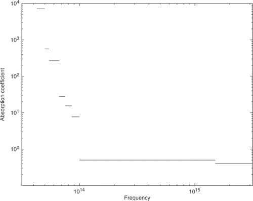
The used physical parameters are collected in table 1. The absorption coefficient corresponds to some realistic type of glass and is taken from 8. It is visualized in figure 1. The time t_f, up to which the measurements are available, has a strong influence on the solution of the inverse problem. If t_f is chosen too small, then the reconstruction is rather poor. The same happens if t_f is too big. The optimal value for t_f depends on the involved physical parameters. The value from table 1 is a good choice for the considered example.

Figure 1. Visualization of the absorption coefficient.

Table 1. Physical parameters that were used for numerical results.

k	νk(10^13Hz)	κk(m^-1)
1	4.28	7136.1
2	5	567.32
3	5.45	267.98
4	6.66	27.98
5	7.5	15.45
6	8.57	7.7
7	9.99	0.5
8	149.9	0.4
cm: 1000 J(kg K)^−1; ρm: 2500 kg m^−3; kh: 1 W(mK)^−1; ng: 1; Ta: 300 K; l: 0.01 m; tf: 25 s

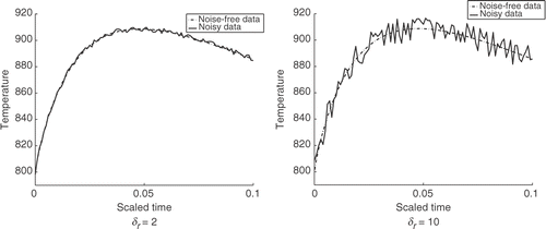
We present numerical results that show the typical behavior of the method. The chosen initial temperature has a symmetric profile with values between 800 and 1200 K. Noise-free and noisy data for two different noise levels δ_r are shown in figure 2.

Figure 2. Noisy data that were used in computations. The noise-to-signal ratio, i.e., ‖ y-y_δ ‖ /‖ y_δ ‖, is: 9.8· 10^-4 for δ _r=2, 5.52· 10^-3 for δ _r=10.

Remark 1 In some applications, e.g., in image processing, reconstruction of nonsmooth solutions may be important. It is not the case in our problem. Since in practice the material has already been involved in the cooling before the measurements start, we may expect the initial temperature to be a smooth function.

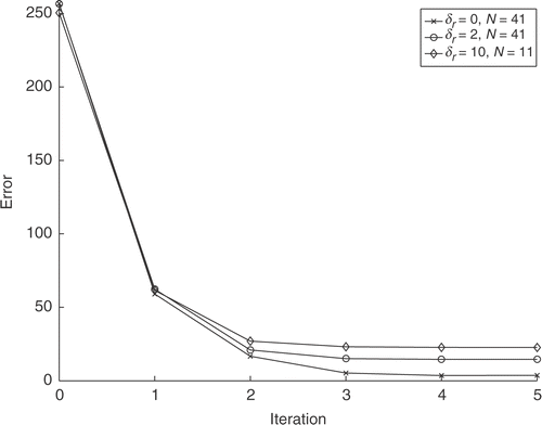
Let be the sequence of approximations for a fixed discretization N. The errors with respect to the iteration number k for (δ _r=0,N=41), (δ _r=2,N=41), and (δ _r=10,N=11) are plotted in figure 3. One observes fast convergence of approximating sequence . Note that the smaller the noise level, the better is the final approximation.

Figure 3. The iteration error for different discretization and noise levels.

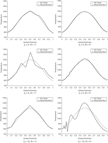
The discretization parameter N has a significant influence on the reconstruction. In fact, the discretization brings additional noise. First, instead of the operator equation (14) we solve the discrete system of (15). Secondly, the functions and the scalar products in (15) can be computed only approximately. Thus, the discretization and the noise need to be balanced, which is illustrated by the numerical examples in figure 4. If no random noise (i.e., δ _r=0) is added, then increasing N will give better results. In the presence of the noise the numerical results suggest, that there is a strong nonmonotonic dependence of the reconstruction accuracy on the discretization. Thus, criteria are needed for choosing the discretization adaptively depending on the data noise.

Figure 4. Reconstructions for different random noise and different discretization. The data is available at z_b = 0, i.e., the left end.

5. Conclusion and outlook

We presented a fast derivative-free iterative method of the initial temperature reconstruction for the nonlinear heat equation. Its numerical performance was checked for the 1D model of the glass plate cooling. The application of the method to the real data is the next step. Another issue of practical importance is treating multidimensional (2D, 3D) cooling processes. With respect to the further theoretical investigations, a rigorous convergence analysis and development of criteria for the choice of discretization parameters can be named. Some results concerning the first issue can be found in 18.

Finally, we would like to point out a possible extended formulation of the inverse problem. In the considered model, we have assumed that the law for the boundary heat flux is known equation (4). In some situations, however, this is not the case, see e.g., 19. Thus, it could be of interest to investigate the problem of recovering the initial temperature and the boundary heat transfer law simultaneously. For such a problem, additional data may be required.

Acknowledgments

This work has been supported by the Kaiserslautern Excellence Cluster “Dependable Adaptive Systems and Mathematical Modeling” and the DFG via contract PI 408/3-1.

Notes

¹ In general, the absorbtion coefficient depends additionally on the direction and temperature. This dependence often can be neglected for glass 11.

References

- Thömmes, G, Pinnau, R, Seaid, M, Götz, Th, and Klar, A, 2002. Numerical methods and optimal control for glass cooling processes., Transport theory and Statistical Physics 31 (2002), pp. 513–529.
- Pinnau, R, and Thömmes, G, 2004. Optimal boundary control of glass cooling processes., Mathematical Methods in the Applied Sciences 27 (2004), pp. 1261–1281.
- Nguyen, KT, and Prystay, M, 1999. An inverse method for estimation of the initial temperature profile and its evolution in polymer processing., International Journal of Heat and Mass Transfer 42 (1999), pp. 1969–1978.
- Nguyen, KT, and Bendada, A, 2000. An inverse approach for the prediction of the temperature evolution during induction heating of a semi-solid casting billet., Modelling and Simulation in Material Science Engineering 8 (2000), pp. 857–870.
- Justen, L, 2002. "An inverse heat conduction problem with unknown initial condition". In: Diploma thesis. Universität Kaiserslautern; 2002.
- Dahlke, S, and Maaß, P, 2003. An outline of adaptive wavelet Galerkin methods for Tikhonov regularization of inverse parabolic problems. Presented at Recent Development in Theories and Numerics. Proceedings of the International Conference on Inverse Problems. Hong Kong, China, 9–12 January, 2002.
- Viskanta, R, and Anderson, EE, 1975. Heat transfer in semitransparent solids., Advances in Heat Transfer 11 (1975), pp. 317–441.
- Neunzert, H, Siedow, N, and Zingsheim, F, 2001. "Simulation of the temperature behaviour of hot glass during cooling". In: Cumberbatch, E, and Fitt, A, eds. Mathematical Modeling: Case Studies from Industry. Cambridge: Cambridge University Press; 2001. pp. 181–198.
- Brinkmann, M, and Siedow, N, 2002. "Heat transfer between glass and mold during hot forming". In: Loch, H, and Krause, D, eds. Mathematical Simulation in Glass Technology. Berlin: Springer-Verlag; 2002. pp. 239–262.
- Modest, MF, 1993. Radiative Heat Transfer. New York: McGraw–Hill ; 1993.
- Lentes, FT, and Siedow, N, 1999. Three-dimensional radiative heat transfer in glass cooling processes., Glass Science and Technology—Glastechnische Berichte 71 (1999), pp. 188–196.
- Laitinen, M, and Tiihonen, T, 2001. Conductive-radiative heat transfer in grey materials., Quarterly of Applied Mathematics 59 (2001), pp. 737–768.
- Asllanaj, F, Jeandel, G, Roche, JR, and Schmidt, D, 2003. Existence and uniqueness of a steady state solution of a coupled radiative-conductive heat transfer problem for a non-grey anisotropically and participating medium., Transport Theory and Statistical Physics 32 (2003), pp. 1–35.
- Asllanaj, F, Jeandel, G, Roche, JR, and Lacroix, D, 2004. Transient combined radiation and conduction heat transfer in fibrous media with temperature and flux boundary conditions., International Journal of Thermal Science 43 (2004), pp. 939–950.
- Engl, HW, Hanke, M, and Neubauer, A, 1996. Regularization of Inverse Problems. Dordrecht: Kluwer Academic Publishers; 1996.
- Pereverzev, S, and Schock, E, 2000. Morozov's discrepancy principle for Tikhonov regularization of severely ill-posed problems in finite-dimensional subspaces., Numerical Functional Analysis and Optimization 21 (2000), pp. 901–916.
- Tikhonov, AN, and Glasko, VB, 1965. Use of the regularization method in non-linear problems., USSR Computational Mathematics and Mathematical Physics 5 (1965), pp. 93–107.
- Pereverzyev, SS, Pinnau, R, and Siedow, N, 2006. Regularized fixed-point iterations for nonlinear inverse problems., Inverse Problems 22 (2006), pp. 1–22.
- Engl, HW, Fusek, P, and Pereverzev, SV, 2005. Natural linearization for the identification of nonlinear heat transfer laws., Journal of Inverse Ill-Posed Problems 13 (2005), pp. 1–16.