Determination of the distribution of the number of specular points of a random cylindrical homogeneous Gaussian surface

Abstract

Statistical characteristics of light reflected by the rough random cylindrical homogeneous Gaussian surface are being investigated by using the method of specular points. The inverse problem, in the form of a Fredholm integral equation of the first kind for determining the distribution of the number of specular points from the known reflected radiance distribution, is formulated. The kernel of this equation is determined by the characteristic function of the distribution of radii of curvature in specular points, derived by Gardashov. The validity of the obtained original formulas is controlled by numerical simulations.

Keywords:

• Specular points
• Radius of curvature
• Gardashov's distribution
• Gaussian surface
• Inverse problem
• Integral equation

1. Formulation of the problem

It is well known that, in the approach of geometrical optics, the statistical characteristics of the light reflected by a random sea surface are determined by statistical characteristics of mirror reflection (or specular) points 1, 2. Let a cylindrical homogeneous Gaussian surface z = ζ(x), (⟨ζ(x)⟩ = 0 , σ₀² = ⟨ζ²(x)⟩ ,  σ₁² = ⟨ζ'²(x)⟩ , be illuminated by a parallel light beam incident along a unit vector and let surface segment with a horizontal length L be observed along a unit vector (figure 1). Then, according to the approach called the method of specular points, a random realization of the radiance (surface reflectance), r, of light reflected from surface is given as the sum of contributions of all specular points (SP) 3: (1)

Figure 1. The geometry of problem.

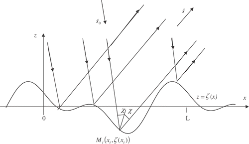
Here, K = πV(χ) cos χ/2|s_0z|s_z, where V(χ) is the Fresnel reflection coefficient at the local incident angle χ; N_L is the number of SP in interval [0, L]; |ρ_i| = (1 + r²)^3/2/|ζ″(x_i)| is the radii of curvature at the SP, M_i (x_i, ζ(x_i)), of the surface z = ζ(x) with a slope: (2)

The specular points M_i (x_i, ζ(x_i)) are determined as the solutions of equation: (3)

The number N_L in sum (1) is the number of solutions of equation (3) falling on the observed part of surface z = ζ(x).

Introducing dimensionless radii of curvature (4) where (5) is the average of radii of curvature |ρ_i| at the SP 4, and denoting (6) the formula (1) can be rewritten: (7)

In the expression (7), the random quantities are the dimensionless radii of curvature X_i and the number of SP, N_L. The expression (7) assumes that the light waves reflected by adjacent SP are incoherent. This assumption will be justified if surface rms deviation is σ₀ ≫ λ.

For the average radiance from expressions (1) and (7) we have (appendix, Theorem 1): (8) where, , is the average number of SP per unit length. (Note that we fix the averaging by angle brackets). As it can be shown (see formula (14)), (9) and, consequently, (10)

This is a well-known result of method of stochastically distributed areas, which states that the angular distribution of the average radiance reflected from the surface is governed by the distribution W(γ) of surface slopes γ. Thus, the average radiance evaluated by the method of specular points coincides with the average radiance evaluated by the method of stochastically distributed areas.

The main goal of this article is deducing the integral equation for determining the distribution of the number of SP from the known reflected radiance distribution.

2. Distribution of the radii of curvature

The distribution of radii of curvature of rough random cylindrical homogeneous Gaussian surface z = ζ(x) at the SP with slopes ζ′(x) = γ ≡ const. is obtained by the following way: using the results of classical works of Rice 5, 6, for average value, , of number of SP per unit length, we can write: (11) where, by W₂(ζ′, ζ″), the joint probability distribution function of derivatives ζ′(x) and ζ″(x) is denoted. The conditional probability distribution function W_c(ζ″\vert γ) of derivative ζ″(x) at the SP, ζ′(x) = γ ≡ const., is expressed by formulae: (12)

Then for the probability distribution function, W_ρ(|ρ|), of the radii of curvature |ρ| = (1 + γ²)^3/2/|ζ″| at the SP ζ′(x) = γ ≡ const. we obtain: (13)

Using the fact that successive derivatives ζ′(x) and ζ″(x) are statistically independent, we have W₂(ζ′, ζ″) = W(ζ′)W₁(ζ″) and for average value of |ρ| we found: (14)

Particularly, for Gaussian surface, i.e. when (15) from (13) and (14) we have: (16) and (17) consequently. The distribution (16) expressed in terms of dimensionless radii of curvature, , is given by the formula: (18) The Gardashov's distribution (18) does not contain any parameter; consequently, it is universally valid for any homogeneous Gaussian surface z = ζ(x). It can be easily seen that and ⟨X²⟩ = +∞. Note that the distribution of the dimensionless radii of curvature with sign, , is symmetric and it is: (19)

3. Distribution of the radiance of reflected light

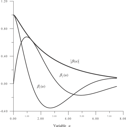
The distribution function W_r(r) of the radiance r can be determined through the characteristic function β(u) of the distribution W_x(X) and the distribution function W_N(N_L) of the number of SP, N_L. From (18) for W_x(X), we obtain the expression for the characteristic function β(u) of the random quantity X: (20)

As we see, the integral converges uniformly on u in (−∞, +∞). In figure 2, the real β₁(u), imaginary β₂(u) parts and the module |β(u)| of characteristics function β (u) are represented.

Figure 2. The real β₁(u), imaginary β₂(u) parts and module |β(u)| of characteristics function β(u).

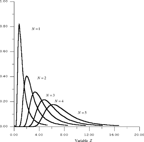
It can be shown (appendix, Theorem 2), that the PDF of the sum (21) under the assumption of independence X₁, X₂, …, X_N, can be expressed in terms of module and argument ϕ(u) = arg β(u) = arctan(β₂(u)/β₁(u)) of characteristic function β(u) as follows: (22)

If we denote (23) then (22) can be rewritten as: (24)

In the special case when W_N(N_L) = δ(N_L − N) from (24), we have (25) which specifies a mean of function G(Z, N), as the distribution of Z when the number of SP, N_L, in the sum (21) is fixed and equal to N. In addition, if N_L ≡ N = 1 then Z = X and G(X, 1) = W_x(X). The graphs of G(Z, N) are given in figure 3. The function G(Z, N) has also a property of universality for any homogeneous Gaussian surface z = ζ(x), as the distribution W_x(X) and its characteristic function β(u).

Figure 3. The special function G(Z, N) for different values of N.

Note that the strong theoretical estimation of the correlations between X₁, X₂, …, X_N is a difficult problem, in spite of the rough estimation of correlation that can be made, for example, in the case of Gaussian correlation function: . Here l₀ is a radius of correlation, which is defined from: B₀(l₀)/B₀(0) = (1/e). Then the radii of correlation of ζ′(x) and ζ″(x) are: l₁ ≈ 0.51l₀ and l₂ ≈ 0.39l₀, respectively. For Gaussian surface z = ζ(x) from (11) we have: . Using the relations and , at γ = 0 we obtain: . Then the mean distance between SP is: . As we see, is greater than the radius l₂. Therefore we can expect for some weak correlations between X₁, X₂, …, X_N.

The assumption of independence N_L from X₁, X₂, …, X_N, is not incredible and may be explained also. Indeed, the more of all X₁, X₂, …, X_N, the less N_L. But, due to weak correlations between X₁, X₂, …, X_N the probabilities of this event (becomes simultaneously greater values of all X₁, X₂, …, X_N for an any realization of surface z = ζ(x)) must be very small.

Note that formula (8) contradict to results in 9, 10. The explanation of this contradiction is given in appendix.

4. Simulation and analysis

We used simulations to test the correctness of the derived analytical formulas. The random cylindrical homogeneous Gaussian surface z = ζ(x) is represented as the sum of harmonics (26) where the phases ϵ_n are uniformly distributed over the interval [0, 2π] and the amplitudes c_n are determined from the energy spectrum . The correlation function of surface z = ζ(x) is taken as Gaussian. Then the spectrum is also Gausssian. The equation (3) that determines the SP, M_i (x_i, ζ(x_i)), of the surface z = ζ(x) described by the formula (26), takes the form (27)

We find numerically all the roots x_i of last equation falling on interval [0, L]. Then we calculate radii of curvature |ρ_i| at the SP, (x_i, ζ(x_i)). This procedure is repeated for an ensemble of surface realizations {z = ζ(x)}. Thus we obtain the set of realizations of the radii of curvature {|ρ|}at the SP, the set of realizations of the numbers of SP, {N_L}, in the horizontal length L, and the set of realizations of the radiance of light {r} reflected from the surface z = ζ(x) with the horizontal length L. From this sets we construct the histograms of the distributions: W_ρ(|ρ|)–the radii of curvature |ρ|, W_N(N_L)–the number of SP, N_L, and W_r(r)–the radiance r.

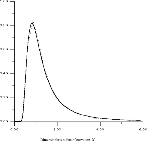
In figure 4, the distribution of radii of curvature W_x(X) obtained by the theoretical formula (18) and its histogram are represented.

Figure 4. The distribution of radii of curvature W_x(X) (solid curve) and its histogram (dashed curve).

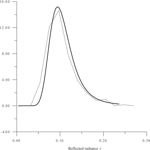
Figure 5 shows the distribution obtained by using the theoretical formula (24) (with a priori taking normal distribution W_N(N_L)) and its histogram. Probably, the main courses of the difference in theoretical and simulated curves in figure 5 are: (1) the correlations between X₁, X₂, …, X_N, which are taken into account automatically in simulation and are neglected in theoretical formula, (2) the computing errors, which must be essentially less than the effect of correlations, because double precision in computing was used. Note that closest of these curves indicates either the weak correlations between X₁, X₂, …, X_N, or the small effect of those correlations to distribution W_r(r).

Figure 5. The distribution of reflected radiance W_r(r); solid curve–theoretical, dashed curve–histogram.

5. Inverse problem for determination of the distribution of the number of SP

The formula (24) can be considered as an integral equation with respect to unknown function W_N(N_L). It means that on the known function W_Z(Z) the unknown function W_N(N_L) can be determined by solving the integral equation (24). The kernel of this equation G(Z, N) is a good function. For fixed value N, the function G(Z, N) has one maximum and tends to zero very rapidly and slowly at Z → 0 and Z → +∞, consequently (figure 3).

As it follows from (1), (6–8) and (21), if the average of radii of curvature, (or average number of SP ), is defined somehow (i.e., a priori known), then the distribution W_Z(Z) of can be simply derived from W_r(r) as: (28) since is a known quantity.

Thus, equation (24) formulates an inverse problem, in the form of a Fredholm integral equation of the first kind, for determining the distribution of the number of specular points, W_N(N_L), from the known distribution of reflected radiance, W_r(r). It is well known that this problem is ill-posed and its solution requires a special method of regularization 9.

Note that the direct solution of equation (24), by transforming it to the system of linear equations (without any regularization algorithm), gives good results when number of SP, N_L, is about five. For large numbers, N_L, the system of linear equations becomes ill-posed and needs regularization.

Actually, when we want to derive W_N(N_L) from W_r(r), the uncertainty arises if a priori are not known as and . The uncertainty can be removed by using the fact that for different N the distribution of Z, i.e. the curves G(Z, N) are essentially different on form. For instance, we can define as the value of N which gives the minimum to the function: (29) where is determined from (8) and .

6. Conclusions

When considering the light reflection from a rough surface, the more general quantity of interest is distribution of reflected light intensity. In this article, the analytical solution of this problem for cylindrical homogeneous Gaussian surface z = ζ(x) is obtained under the assumption: “there are no correlations between radii of curvature at specular points and number of specular points”. The degree of validity of this assumption for different types of correlation functions must be investigated. The closest of theoretical and simulated curves of the distribution W_r(r) (figure 5) tells us that the effect of correlation is small, at least for a Gaussian correlation function. The result of simulations, in the wide range of parameters l₀, σ₀, γ, shows the workability of the formulated inverse problem.

The analogous problem can be formulated and solved for a 3D random homogeneous Gaussian surface z = ζ(x, y) (such as a wavy sea surface) for which the convenient expression for the distribution of Gaussian curvature at SP is known 10. In this case the solution of the inverse problem may be examined by the natural experiments, also, for instance, by using the ensemble of digital images of Sun glitters.

The future aim of author is to choose an appropriate algorithm of regularization and the application of this method to define the number of SP (glitters) and radii of curvatures of sea surface from the remote sensing dates.

Appendix

A1. Proof of the formula (8)

Theorem 1

Let in the sum (30)

a.	the quantities X1, X2, …, XN and N are random variables;
b.	X1, X2, …, XN has the same PDF and finite mathematical expectation of E(X);
c.	N is a positive integer (N ≥ 1) with finite mathematical expectation of E(N) and PDF of P(N);

Then, the mathematical expectation of the sum is finite and is: (31)

Proof

By using the formula of total mathematical expectation we have:

Here E(Z|N = n) is conditional mathematical expectation of Z, i.e. at the fixed N = n.

Thus (A2) is correct.

The formula (A2) coincides with , from which follows (8).▪

Note: As we can see from this proof the independence of random variables X₁, X₂, …, X_N, N is not required.

A2. Proof of the formula (22)

Theorem 2

Let in the sum

a.	the random variables X1, X2, …, XN > 0, are independent and has the same PDF, Wx(X);
b.	the random variable N is positive integer (N ≥ 1) and has PDF, WN(N).

Then PDF of random variable Z is given by (32) where β(u) is a characteristic function of distribution W_X(X);

ϕ(u) is an argument of β(u).

Proof

Let the joint PDF of random variables Z and N is W_ZN(Z, N), and conditionally PDF is W_ZN(Z|N). Then (33) and (34)

If we denote the joint PDF of random variables X₁, X₂, …, X_N by then from independence of X₁, X₂, …, X_N we have:

Characteristic function, Θ(u), of the distribution of random variable Z at the fixed N (i.e. of the PDF W_ZN(Z|N)) is: (35)

Thus (36)

Then PDF W_ZN(Z|N) of random variable Z at the fixed N, is expressed in terms of Θ(u) by: or (37)

As can be seen, the characteristic function has properties: Then . Therefore, in (A8), first integrand is even function and second integrand is odd function. Using this fact we have: (38)

Substituting (A9) in (A5), we obtain (A3).

As we see from (A9), the function G(Z, N), which is defined on (23), coincides with PDF, W_ZN(Z|N).▪

A.3. On contradiction between the formula (8) and results in papers Barrick 7, and Barrick and Bahar 8

The origin of contradiction between the equation (8) in present article and its 3D analog–the equation (6) in 8, is hiding the different meanings of N_L in present article and N in equation (6) from 8. The quantity N_L has a clear geometrical sense: N_L is the number of SP in interval [0, L] for a given (any considered) realization z = ζ(x). But N in 8 has other meaning: N is the density of SP per unit area with fixed second derivatives ζ_xx, ζ_yy, ζ_xy (in 2D case, N is the density of SP per unit length with a fixed second derivative ζ″). However, , if N is for 2D case.

As we can see, in my consideration, no meanings have the expressions N_L·|ρ| and (where, |ρ| is a radius of curvature at SP), because for any realization z = ζ(x) the set of radii and N_L are appeared, but not indefinite one |ρ| at SP. Therefore, we can speak only about the correlation between N_L and any fixed |ρ_i|, i = 1, 2, …, N_L from the set . I think this correlation must be weak, as it's explained earlier in text. In my consideration the averaging of N_L is performed on the ensemble of realization of surface {z = ζ(x)} and the averaging of |ρ| is performed on the whole set within the ensemble {z = ζ(x)}.

But in 8 definite meanings have the expressions N·|ρ| and , where the averaging is performed on the ensemble of realization {z = ζ(x)}. Indeed, the random variables N and |ρ| in 8 are dependent: the more |ρ|, the less N.

However, the conclusion in 8 (which follows from equations (6) and 7 in 8), that , is incorrect if the averaging ⟨|r_1pr_2p|⟩ is performed on the whole set of SP. When the averaging is performed on the whole set of SP, the equation (7) in 8 is correct. It follows from Longuet-Higgens 11 results.

For density of SP per unit area, D_sp, in 11 the following equation is obtained (the symbols and the numeration of equation–on 11): (39) where (40) (41)

The conditional probability distribution of ζ₁, ζ₂, ζ₃ at SP, i.e. where ζ₄, ζ₅ have given constant values ζ₄ = γ_x = const., ζ₅ = γ_y = const is defined by: (42)

For average of we found: Thus, (43)

In 8 symbols equation (A10) is: (44)

From equation (A11) and equation (16) in 8 we obtain: (45)

Hereby, if the averaging ⟨|r_1pr_2p|⟩ is performed according to above-mentioned procedure of 11 (but not on equation (15) in 8, where the integrand has singularity and on equation (10) in 7, which is approximation) then the equation (A12) is correct.

Note that equation (A10) or (A11) is the 3D analog of equation (9) in present article.

References

- Kravtsov, YA, and Orlov, YI, 1990. Geometrical Optics. Berlin, Heidelberg: Springer Verlag; 1990.
- Bass, FG, and Fuks, IM, 1978. Wave Scattering from Statistically Rough Surfaces. Oxford: Pergamon; 1978.
- Shifrin, KS, and Gardashov, RG, 1985. Model calculations of light reflection from the sea surface, Izvestiya Akademii Nauk SSSR. Fizika Atmosfery i Okeana 21 (2) (1985), pp. 162–169.
- Gardashova, TG, and Gardashov, RG, 2001. Simulation of statistical characteristics of light reflected from the sea surface, Izvestiya, Atmospheric and Oceanic Physics 37 (1) (2001), pp. 67–77.
- Rice, SO, 1944. Mathematical analysis of random noise, Bell System Technical Journal 23 (3) (1944), pp. 282–332.
- Rice, SO, 1945. Mathematical analysis of random noise, Bell System Technical Journal 24 (1) (1945), pp. 46–156.
- Barrick, D, 1968. Rough surface scattering based on the specular point theory, IEEE Transactions on Antennas and Propagation AP-16 (4) (1968), pp. 449–454.
- Barrick, D, and Bahar, E, 1981. Rough surface scattering using specular point theory, IEEE Transactions on Antennas and Propagation AP-29 (5) (1981), pp. 798–800.
- Tikhonov, AN, and Arsenin, VY, 1977. Solutions of Ill-Posed Problems. Washington: V.H. Winston & Sons; 1977.
- Gardachov, RG, 2000. The probability density of the total curvature of a uniform random Gaussian sea surface, International Journal of Remote Sensing 21 (15) (2000), pp. 2917–2926.
- Longuet-Higgens, MS, 1959. The distribution of the sizes of images reflected in a random surface, Proceedings of the Cambridge Philosophical Society 55 (1959), pp. 91–100.