Equation error approach for elliptic inverse problems with an application to the identification of Lamé parameters

Abstract

The method of equation error can be posed and analyzed in an abstract setting that encompasses a variety of elliptic inverse problems, in which a coefficient in an elliptic partial differential equation is to be estimated from a measurement of the solution to a boundary value problem. Stability in the presence of measurement error is obtained by regularization, and since the abstract setting admits the use of total variation regularization, rapidly varying or even discontinuous coefficients can be estimated. The proposed method effectively identifies Lamé' parameters in the system of linear isotropic elasticity.

Keywords:

• Equation error method
• Stability analysis
• Lamé coefficients
• Linear elasticity
• Inverse problem
• Regularization
• Total variation

AMS Subject Classifications:

• 35R30
• 65N30

1. Introduction

In recent years, the field of inverse problems has emerged as among one of the most active branches of applied and industrial mathematics. This is partly due to the ever-growing number of real-world situations that can be modeled and studied in a unified framework as inverse problems. The theoretical aspects of inverse problems are challenging and require a fine blending of various branches of mathematics. Recent developments in this field have prompted a need to study nonsmooth optimization problems in nonreflexive Banach spaces, an issue that is addressed in this article.

The prototypical elliptic inverse problem arises in the context of the following elliptic boundary value problem (BVP): (1) (2) Here Ω is a suitable domain in ℝⁿ and ∂Ω is its boundary. The above BVP models several interesting real-world problems and has been studied in great detail 11, 13, 17, 18. For instance, u = u(x) may represent the steady-state temperature at a given point x of a body; then a would be a variable thermal conductivity coefficient and f the external heat source. The system (1) also models underground steady state aquifers in which the coefficient a is the aquifer transmissivity coefficient, u is the hydraulic head and f is the recharge. In either context the direct problem is to find u given the coefficient a and the source term f. On the other hand, the inverse problem is to identify the coefficient a, provided that a measurement of u is known. For details of this as well as other inverse problems, see 2, 12, 15, 19, 25, 27, 34.

A number of approaches to the aforementioned inverse problem have been proposed in the literature; most involve either regarding (1a(1) ) as a hyperbolic PDE in a or posing an optimization problem whose solution is an estimate of a. The work by Richter 32, who used a finite difference scheme to solve for a, is an example of the first approach. There are a variety of ways to pose an optimization problem for a, including the equation error method, which is the subject of this article.

The output least-squares (OLSs) approach for estimating a seeks to minimize the functional defined by an appropriate norm. Here z is the data (the measurement of u) and u(a) is the solution of (1) for a. For instance, Falk 15 analyzed the case of the L² norm applied to the scalar problem (1). Recently, Zou 35 (see also 7), and Knowles 25 have independently proposed using a coefficient-dependent norm in the OLS setting. The present authors 20 showed how to extend this idea to more general elliptic inverse problems, such as the problem of estimating the Lamé moduli in the equations of isotropic elasticity.

The equation error method (cf. 1, 24), consists of minimizing the functional where H⁻¹(Ω) is the topological dual of H0¹(Ω) and z is the data (the measurement of u). Kohn and Lowe 26 proposed a variational method that combines features of the OLS and equation error methods. Ito and Kunisch 22 developed an augmented Lagrangian algorithm to solve the OLS problem by treating the PDE as an explicit constraint. This approach has been extended in 3, 9.

The primary objective of this study is to analyze the equation error approach from an abstract point of view and use it for the numerical identification of the Lamé parameters in the following system that describes the response of an isotropic membrane or body to a traction applied to its boundary: (3) (4) The domain Ω is a subset of ℝ² in the case of a membrane or ℝ³ in the case of a body, and ∂Ω = Γ1 ∪ Γ2 is a partition of its boundary. The details of the above model will be supplied in section 3. At this point we only state that the direct problem for (2) is to compute the vector-valued displacement u, given that h and the coefficients μ and λ are known. We are interested in the inverse problem of estimating the nonconstant coefficients μ and λ, given h and a measurement of u.

An excellent reference for the theory of the direct problem is the text by Duvaut and Lions 11. The inverse elasticity problem has been studied from the theoretical standpoint, for example in 5. Recently, interesting applications, such as elasticity imaging, have sparked a new interest in these problems (see 23, 28, 30, 31 and the references therein). More specifically, it is possible, using ultrasound, to measure interior displacements in human tissue (for example, breast tissue). Since cancerous tumors differ markedly in their elastic properties from healthy tissue, it may be possible to discover and locate tumors by solving an inverse problem for μ and λ.

This work is divided into four sections. Section 2 describes the equation error approach in an abstract setting. A minimization problem is studied in a nonreflexive Banach space and some stability estimates are given. Convergence analysis is given for the discretized minimization problem. Section 3 deals with the application to isotropic elasticity. Numerical results are given in section 4.

2. Equation error approach

Assume that V is Hilbert space and B is a Banach space that is continuously embedded into a Banach space L. Assume that another Banach space is compactly embedded into L. Moreover, we assume that there are constants C1 > 0 and C2 > 0 such that for all x ∈ A, where is the set of admissible coefficients. We assume that A is convex, and closed with respect to ‖·‖L. By ψ : A → ℝ we denote a proper convex positive functional that is lower-semicontinuous with respect to ‖·‖L and uniformly bounded over A. We assume that T : B × V × V → ℝ is a trilinear form with T(a, u, v) symmetric in u, v, and that there exist positive constants k1 and k2 such that (5) (6) Finally, we assume that m is a bounded linear functional on V. Then, for any a ∈ A, it follows from the Riesz representation theorem that the following variational equation has a unique solution u ∈ V: (7)

In the present setting, the inverse problem associated with the direct problem (4(7) ) is the following: Given some measurement of u, say z, estimate the coefficient a which together with u makes (4(7) ) true.

By the Riesz representation theorem, there is an isomorphism E : V → V* defined by For each (a, u) ∈ A × V, T(a, u, ·) − m(·) ∈ V*. We define e(a, u) to be the pre-image under E of this element:

For a fixed z ∈ V, we consider the following minimization problem. Find a* ∈ A by solving (8)

In (5(8) ), ψ corresponds to a nonquadratic regularization (often a seminorm), a technique which has received much attention recently to identify coefficients that vary rapidly or are discontinuous. In practice the parameter α is chosen to be quite small, and hence the quadratic term α‖a‖² plays a purely technical role; it ensures the uniqueness.

The equation error approach has two advantages over the OLS approach. Firstly, J is convex, which ensures global solvability. Secondly, the approach is easily implementable for a numerical solution. A deficiency of the approach is due to the fact that it relies on differentiating the data and hence is sensitive to the error in the data. However, in 21 we have shown, in the context of the scalar BVP, that a simple data smoothing alleviates this shortcoming quite effectively.

We begin with the following existence result.

Theorem 2.1

Assume that for an → a in L, we have e(an, z) → e(a, z) in V. Then the minimization problem (5(8) ) has a unique solution.

Proof

Since J(a) ≥ 0 for all a ∈ A, there exists a minimizing sequence {ak} in A such that It follows that {J(ak)} is bounded above and hence {ak} is bounded above in ‖·‖L. In view of the assumption it remains bounded in Therefore, {ak} has a subsequence which, due to the compact embedding of into L, converges in L, to some a* ∈ A. (Throughout this work we will use the same notation for a sequence and its subsequences.) Notice that in view of the assumptions on e(·, ·) we have e(ak, z) → e(a*, z). Consequently This confirms that a* is a solution of (5(8) ). The uniqueness follows from the strong convexity of J.▪

We remark that the functional J being convex, a necessary and sufficient optimality condition for (5(8) ) is a variational inequality of the second kind (due to the nondifferentiable term ψ(·)), involving the Fréchet derivative of J0(·), defined by where e1 is given by ⟨e1(a, z),v⟩ = T(a, z, v) for all v ∈ V.

A crucial step in the above proof is the existence of a subsequence that converges in ‖·‖L. This is achieved through the quadratic regularization term and the assumptions that and that the space is compactly embedded into the space L. Therefore, if we take α = 0 then we should assume that the set A is bounded in

Before any further advancement we pause to justify the abstract setting described above. We choose an inverse problem of identifying the coefficient a in a Helmholtz equation 6 to explain the basic ideas behind the assumptions. A more involved case of an inverse problem in isotropic elasticity problem will be discussed later.

We consider the following BVP: (9) (10)

The above assumptions are motivated by the space of functions of bounded variation (BV). Recall that the total variation of f ∈ L¹(Ω) is defined by where ‖·‖ represents the Euclidean norm of a vecto.1 If f ∈ L¹(Ω) satisfies TV(f) < ∞, then f is said to have bounded variation, and the space BV(Ω) is defined by The norm on BV(Ω) is ‖ f ‖BV(Ω) = ‖ f ‖L¹(Ω) + TV( f ), where TV(·) is the BV-seminorm on BV(Ω). It is known that TV(·) is convex and lower-semicontinuous with respect to ‖⋅‖L¹(Ω) 14, 16.

We set V = H0¹(Ω), B = L^∞(Ω), L = L¹(Ω), and ψ(a) = TV(a). Then the embedding assumptions follow from the following properties of BV(Ω) and L^∞(Ω):

1.	L∞(Ω) is continuously embedded in L1(Ω).
2.	BV(Ω) is compactly embedded in L1(Ω).

We define the set of admissible coefficients as follows: where c1, c2 and c3 are constants. Clearly, A is bounded in

The trilinear form T and the functional m are based on the variational form for (1), which reads: Define T(a, u, v) = ∫Ω[a∇u∇v + uv] and m(v) = ∫Ω fv.

Properties (3a(5) ) and (3b(6) ) are easy to verify. Moreover, for (a,z)∈A × H0¹(Ω), the element e(a,z)∈H0¹(Ω) is defined by: It remains to prove that for in L¹(Ω). Indeed, we have Subtracting the above two equations and setting yield This, in view of the Lebesgue-dominated convergence theorem, confirms that .

See 4,8,10 and 33 for interesting results on the use of total variation regularization. Let us now return to the abstract framework. Let z ∈ V be the exact data and let zδ ∈ V be perturbed data satisfying ‖zδ − z‖ ≤ δ. We consider the following problem: find aδ ∈ A by solving (11)

The following stability result is motivated by a result of Nashed and Scherzer 29.

Theorem 2.2

Assume that for an → a in L, we have e(an, z) → e(a, z) in V. Then any sequence {aδ}, where aδ is the unique solution of (7), converges to the minimizer of (5(8) ) as δ → 0.

Proof

We will first show that the sequence {aδ} ⊂ A is uniformly bounded. Indeed, it follows from the definition of aδ that for an arbitrary b ∈ A, we have where c and M are constants. This ensures the existence of a subsequence of {aδ} which converges, in ‖·‖L, to some We claim that solves (5(8) ). Indeed, in view of the identity for any b ∈ A, we have Therefore, is a minimizer of (5(8) ). However, since is unique, we reach the conclusion.▪

In the above two results, α and β were held fixed. In other words, we have only shown that the perturbed regularized problem converges to the regularized problem. In the following, we study the case when both the regularization parameter and the parameter dictating the error, converge to zero.

More precisely, we consider the following problem: for a fixed n ∈ ℕ, find an ∈ A by solving (12) In this situation, it is necessary to relate the convergence of δn to that of αn and βn. The problem, therefore, is to choose αn, βn appropriately, knowing δn. We assume that and are uniformly bounded and {αn, βn, δn} → 0.

Theorem 2.3

Assume that (a*, z) is a solution of (4(7) ) and (e·, z) is injective. Assume that for an → a in L, we have e(an, z) → e(a, z) in V. Then, there is a subsequence {an}, where an is a solution of (8), that converges to a*.

Proof

We claim that the sequence {an} is uniformly bounded in ‖·‖L. We have implying the boundedness of {an}. Therefore there is a subsequence {an} such that in L.

Furthermore, we have This, in view of the inequality implies that However, since by the assumption e(·, z) is injective, we obtain ▪

The assumption that the map e(·, z) is injective corresponds to the uniqueness of the inverse problem. Richter 32 studies the uniqueness of the inverse problem for the scalar BVP (1). The work of Cox and Gockenbach 9 is devoted to the uniqueness issues for the system of isotropic elasticity. The interested reader may refer to these works for the conditions under which the injectivity hypothesis holds.

2.1. Discrete approximation

To solve either the direct or the inverse problem, discretization is required. In the examples we have in mind, finite element discretization will be used. For the abstract development, we assume that Vk is a sequence of finite dimensional subspaces of V and, for each k, Pk : V → Vk is a projection operator. We assume that Vk and Pk have the property that ‖v−Pk‖V → 0 for all v ∈ V. We similarly assume that Bk is a sequence of finite-dimensional subspaces of B and define Ak = Bk ∩ A. Moreover, we assume that We also consider the finite-dimensional analog ek(·, ·) of the operator e(·, ·), defined as follows: (13) We consider the following discrete minimization problem: find ak ∈ Ak by solving (14) where ψ^(k) is discrete analog of ψ satisfying:

1.	For any a ∈ A, there exists a sequence {ak} ⊂ Ak such that ak → a in L and (15)
2.	For every {ak} ⊂ Ak with ak → a in L, we have (16)

These assumptions will be justified for the concrete cases. We have the following result.

Theorem 2.4

Assume that for an → a in L, T(an, z, v) → T(a, z, v) ∀v ∈ V. Then every subsequence of {ak}, where ak is a minimizer of (10), has a subsequence that converges to a solution of (5(8) ).

Proof

Clearly {ak} is bounded in and hence it has a subsequence which converges, in ‖·‖L, to a* ∈ A. We will show that a* is a solution of (5(8) ). We claim that for ak → a in L, ek(ak, z) → e(a, z), weakly in V. Indeed, for any w ∈ V, we have Since m is continuous, ‖w−Pkw‖V → 0 and T(ak, z,v) → T(a, z, v), we have ⟨ek(ak, z) −e(a, z), w⟩ → 0. Let a ∈ A be arbitrary and let be a sequence which satisfies the condition (11). From the fact that ‖·‖V is weakly lower-semicontinuous, we have In the above, we used the fact that for the inequality holds. Since a is chosen arbitrarily, the theorem is proved. ▪

3. Applications to isotropic elasticity

We are interested in the inverse problem of identifying the Lamé parameters in the following system, which describes the response of an isotropic membrane or body to a traction applied to the boundary: (17) (18) (19) (20) The domain Ω is a subset of ℝ² in the case of a membrane or ℝ³ in the case of a body, and ∂Ω = Γ1 ∪ Γ2 is a partition of its boundary. The vector-valued function u = u(x) represents the displacement of the elastic membrane, and ϵ(u) = (∇u + ∇u^⊤) is the (linearized) strain tensor. The tensor σ is the resulting stress tensor, and the stress–strain law or constitutive equation (13a(17) ) is derived from the assumption that the elastic membrane is isotropic and that the displacement is small (so that a linear relationship holds approximately). The coefficients μ and λ are the Lamé moduli, which quantify the elastic properties of the material. They are constants if the material is homogeneous, and otherwise depend on x ∈ Ω. The boundary conditions (13c(19) ) and (13d(20) ) indicate that the membrane is fixed on Γ1 ⊂ ∂Ω and that a traction h is applied to the rest of the boundary, Γ2.

In order to show the applicability of our general theory, we first fix some notation. The dot product of two tensors A and B, denoted by A · B, is understood as: The L² norm of a tensor-valued function A = A(x) is defined by Moreover, the L² norm of a vector-valued function u = u(x) is defined by while the H¹ norm of u is defined by Finally, the space V (of test functions) is defined by

Green's identity, in the present context, is (21) where σ is assumed to be a symmetric tensor. Using (14(21) ), we now derive the weak form of (13). Multiplying both sides of (13a(17) ) by a test function v, integrating over Ω, and applying (14(21) ) yield Applying (13b–13d(18) ), we obtain the weak form: (22) For given constants k1, k2 satisfying k2 > k1 > 0, we define the following subset of B = L^∞(Ω) × L^∞(Ω): Elements of B will often be denoted by ℓ = (μ, λ). We define a mapping T(·, ·, ·):B × V × V → ℝ by and a functional m : V → ℝ by Clearly the mapping T(·, ·, ·) is trilinear and the functional m(·) is linear and continuous.

By Korn's inquality (see 11, for example), there exists a constant C > 0 such that (23) The following inequality, which holds pointwise in Ω, is easy to establish: (24) Combining (16(23) ) and (17(24) ), we obtain (25) where α = C^† min {2μ+2λ, 2μ}.2 This proves that the bilinear form defining (15) is V-elliptic if min{2μ + 2λ, 2μ} > 0 in Ω. Provided f and h are regular enough, for each (μ, λ) ∈ K, there exists a unique u ∈ V satisfying (15(22) ).

We modify the set of admissible constraints to be and consider the following minimization problem: estimate ℓ* = (μ*, λ*) ∈ K by solving (26) where z is the measurement of u and e(·, ·) is given by:

For simplicity, in (19(26) ) we do not include the quadratic regularization term α‖ℓ‖². We have the following theorem.

Theorem 3.1

The minimization problem (19(26) ) has a global solution.

Proof

In view of Theorem 2.1, it suffices to show that e(ℓn, z) → e(ℓ, z), in V, if ℓn → ℓ in L = L1(Ω) × L1(Ω). Indeed, we have By subtracting the above two equations, and setting v = e(ℓn, z) − e(ℓ, z), we get The proof now follows from the Lebesgue-dominated convergence theorem.▪

For the numerical approximation, we will use the finite element discretization on a family {Th} of triangulations of Ω. We define Ah to be the space of all continuous piecewise polynomials of degree da relative to Th. Similarly, Uh will be the space of all continuous piecewise polynomials of degree du relative to Th, subject to the constraints that the homogeneous Dirichlet boundary conditions on Γ1 are satisfied. The discrete set Kh of admissible coefficients is given by: The next step is to introduce a finite dimensional analog of the map e(a, z) : K × V → V. For any (ah, z) ∈ Kh × Uh, the element eh(ah, z) ∈ Vh is the solution of the variational problem (27)

We consider the following finite-dimensional minimization problem: (28) In the above, TVε(·) is given by where ε = ε(h) > 0 and ε → 0 as h → 0.

We also need to recall that the standard nodal value interpolant satisfies

The following result ensures the convergence of the discrete problem.

Theorem 3.2

The discrete minimization problem (21) is solvable. If is a sequence of its solution, then each subsequence has a subsequence which converges to a minimizer of (19(26) ).

Proof

The existence of minimizers to (21(28) ) follows from Theorem 2.3. The convergence arguments are based on Theorem 2.5. We will construct a sequence satisfying (11). Let be a sequence of minimizers. Clearly this sequence remains bounded in BV(Ω) × BV(Ω). Let be a subsequence which converges to (μ*, λ*) in L¹(Ω) × L1(Ω). For any (μ, λ) ∈ Kh and for constants κ1 > 0 and κ2 > 0, there exists function such that 14, pp. 127, 172] Following the ideas of Zou 35, we define Then, we have .

Moreover and Similarly, we have and

By taking and where Ih(·) is the nodal interpolant, we get By using the lower−semicontinuity of the BV seminorm, we have Now passing {κ1, κ2} → 0, we obtain Therefore, (μ*, λ*) ∈ A solves (19(26) ). The proof is complete. ▪

4. Numerical examples

In this section, we use the equation error approach for numerically identifying the Lamé moduli in linear elasticity. We present two examples, one for smooth Lamé moduli and one for nonsmooth. Finally, by means of an example, we show the effectiveness of the total variation regularization.

4.1. Implementation issues

Recall that Tk is a triangulation on Ω, Ak is the space of all piecewise continuous polynomials of degree da relative to Tk and Uk is the space of all piecewise continuous polynomials of degree du relative to Tk, subject to the constraint that the homogeneous Dirichlet boundary conditions are satisfied. In all of our examples, we use uniform triangulations of the unit square.

In order to represent (20(27) ) in a computable form we proceed as follows. We represent bases for Ak and Uk by {ψ1, ψ2, …, ψm} and {ϕ1, ϕ2, …, ϕn}, respectively. The space Ak is then isomorphic to R^m, and for any a ∈ , we define A ∈ R^m by Ai = a(xi), i = 1, 2, …, m, where {ψ1, ψ2, …, ψm} is a nodal basis corresponding to the nodes {x1, x2, …, xm}. Conversely, each A ∈ R^m corresponds to a ∈ defined by Similarly, u ∈ Uk will correspond to U ∈ Rⁿ, where Ui = u(yi), i = 1, 2, …, n and Here y1, y2, …, yn are the nodes of the mesh defining Uk. (Both Ak and Uk are defined relative to the same triangles, but the nodes will be different if da ≠ du.)

We define F : R^m → Rⁿ to be the finite element solution operator mapping a coefficient a ∈ Ak to the approximate solution v ∈ Uk. Then F(A) = V, where V is defined by (29) and K(A) ∈ R^n×n and F ∈ Rⁿ are the stiffness matrix and load vector, respectively: We also define the matrix L(V) by the condition Recall that for a fixed pair (a, z) ∈ Ah × Uh, the element eh(·, ·) is defined by (30) For eh ∈ Uh, we will have E ∈ ℝⁿ, with Plugging v = ϕi, i = 1, 2, …, n in (23), and performing some simplifications, we get where K is the usual stiffness matrix and Z ∈ ℝⁿ corresponds to the data z. Consequently, we have

The above calculation then leads to Notice that the discrete version of the traditional equation error approach, which incorporates H1 × H¹ regularization 1 gives rise to a convex quadratic functional. As a consequence, the first-order optimality conditions results in a system of linear equations that can be solved quite effectively. However, when regularized, the presence of the nonsmooth term TVβ(A), poses additional difficulties as the above functional is no longer quadratic and hence we must use a nonlinear optimization algorithm. We will need the gradient and the Hessian of J. For δA ∈ ℝ^m, we have and Summarizing,

4.2. Example 1

We consider an isotropic elastic membrane occupying the unit square Ω = (0, 1) × (0, 1). The exact Lamé moduli are λ = 1 and μ = 1 + χS, where S = {(x, y) ∈ S: y ≥ 0.5} and χS is the characteristic function of S. In other words, μ is the discontinuous function whose value is 2 on S and 1 on the rest of Ω. We perform one "experiment" of stretching the membrane by a boundary traction h and measuring the resulting displacement u. 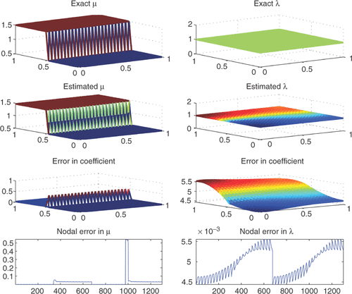The boundary traction chosen is where n is the outward point unit normal to ∂Ω. This traction is applied to the bottom, left, and right edges of the membrane, while the top edge (y = 1) is fixed by a Dirichlet condition. In all finite element computations for this example, we use a sequence of uniform triangulations on Ω. The regularization parameter was chosen to be 10⁻⁵. The coefficients were identified in a finite-dimensional space of dimension of 1301 on a mesh with 2500 triangles. On the other hand the dimension of u was 5050. Since the Lamé moduli are discontinuous, we used BV-regularization. These results seem quite satisfactory. We remark that the discontinuous coefficient was identified quite accurately, except along the line of discontinuity.

4.3. Example 2

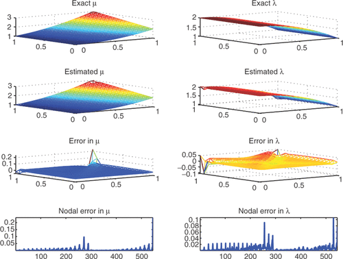
In this example the Lamé parameters are smooth functions. As previously, we consider an isotropic elastic membrane occupying the unit square Ω = (0, 1) × (0, 1), and the exact Lamé moduli are We stretch the membrane by the same boundary traction h employed in the preceding example. As before, the membrane is fixed on the top edge by a Dirichlet boundary condition.

Figure 1. The exact coefficients μ and the estimated μ on a mesh with 2500 elements. The plots also show the element-wise error and the nodal error.

The results of the inversion are shown in figure 2, which show that the coefficients are accurately identified except at the points where the boundary conditions switch from Dirichlet to Neumann. At those points, the estimated parameters show the largest error. The regularization parameter was chosen to be 10⁻⁷. The coefficients were identified in a finite-dimensional space of dimension of 545 on a mesh with 1024 triangles. On the other hand the dimension of u was 2080. Since the Lamé moduli are smooth, we used H¹-regularization. Therefore, the minimization problem was quadratic.

Figure 2. The exact coefficients μ and the estimated μ on a mesh with 545 elements. The plots also show the element-wise error and the nodal error.

4.4. TV versus H¹-seminorm regularization

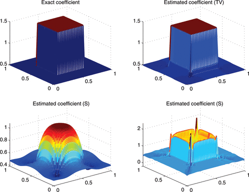
The framework developed in this article applies to both H¹ seminorm regularization and total variation regularization. Although H¹ seminorm regularization is simpler, leading as it does to a convex quadratic objective function, it tends to smooth out discontinuities and rapid variation. The following example illustrates this behavior and the advantages of total variation regularization.

We consider the scalar BVP (1). The exact coefficient now is a(x) = 1 + χS where χ is the indicator function of the set S given by In other words the exact coefficient has constant value 2 on the “square” patch of the domain and 1 on the remaining portion.

Figure 3 shows the results of applying three types of regularization: total variation, H¹ seminorm, and L² norm. These results were obtained on a uniform mesh with 3200 elements. The dimension of the discrete coefficient was 1681 and the dimension of the accurate solution (computed by using cubic finite element functions) was 6241. Figure 3 shows that only total variation regularization is capable of identifying the discontinuity accurately.

Figure 3. Exact coefficient (top left); conefficient estimated by BV regularization (top right); coefficient estimated by H¹ seminorm regularization (bottom left); coefficient estimated by L² norm regularization (bottom right).

Acknowledgements

The authors are grateful to the referees for their careful reading of the article and for the suggested improvements.

Notes

¹ When f belongs to W^1,1(Ω), then it is easy to show (by integration by parts) that TV(f) = ∫Ω‖∇f‖.

² Inequality (17(24) ) is specific to ℝ^†; in a three-dimensional problem, the inequality becomes 2μϵ(v)·ϵ(v) + λtr(ϵ(v))² ≥ min{2μ + 3λ, 2μ} · ϵ(v)·ϵ(v), and therefore α = C²min{2μ + 3λ, 2μ}.

References

- Acar, R, 1993. Identification of the coefficient in the elliptic equations, SIAM Journal on Control and Optimization 31 (5) (1993), pp. 1221–1244.
- Banks, HT, and Kunisch, K, 1989. "Estimation techniques for distributed parameter systems". In: System and Control: Foundations and Applications. Vol. 1. Boston: Birkhauser; 1989.
- Chan, TF, and Tai, XC, 2003. Identification of discontinuous coefficients in elliptic problems using total variation regularization, SIAM Journal of Scientific Computing 25 (2003), pp. 881–904.
- Chan, T, and Tai, XC, 2004. Level set and total variation regularization for elliptic inverse problems with discontinuous coefficients, Journal of Computational Physics 193 (2004), pp. 40–66.
- Chen, J, and Gockenbach, MS, 2002. A variational method for recovering planar Lame moduli, Mathematics and Mechanics of Solids 7 (2002), pp. 191–202.
- Chen, J, Han, W, and Schulz, F, 1994. A regularization method for coefficient identification of a nonhomogeneous Helmholtz equation, Inverse Problems 10 (1994), pp. 1115–1121.
- Chen, Z, and Zou, J, 1999. An augmented Lagrangian method for identifying discontinuous parameters in elliptic systems, SIAM Journal on Control and Optimization 37 (1999), pp. 892–910.
- Chung, ET, Chan, TF, and Tai, XC, 2005. Electrical impedance tomography using level set representation and total variational regularization, Journal of Computational Physics 205 (2005), pp. 357–372.
- Cox, SJ, and Gockenbach, MS, 1997. Recovering planar Lamé moduli from a single-traction experiment, Mathematics and Mechanics of Solids 2 (1997), pp. 297–306.
- Dobson, DC, and Santosa, F, 1996. Recovery of blocky images from noisy and blurred data, SIAM Journal on Applied Mathematics 56 (4) (1996), pp. 1181–1198.
- Duvaut, G, and Lions, JL, 1976. "Inequalities in mechanics and physics". In: Grundlehren der Mathematischen Wissenschaften. Vol. 219. Berlin-New York: Springer-Verlag; 1976.
- Engl, HW, Hanke, M, and Neubauer, A, 1996. "Regularization of inverse problems". In: Mathematics and its Applications. Vol. 375. Dordrecht: Kluwer Academic Publishers Group; 1996.
- Evans, L, 1998. Partial Differential Equations. Providence, RI: American Mathematical Society; 1998.
- Evans, L, and Gariepy, R, 1992. Measure Theory and Fine Properties of Functions. Boca Raton: CRC Press; 1992.
- Falk, RS, 1983. Error estimates for the numerical identification of a variable coefficient, Mathematics of Computation 40 (1983), pp. 537–546.
- Giusti, E, 1984. Minimal Surfaces and Functions of Bounded Variation. Monographs in Mathematics. Vol. 80. Basel: Birkhauser Verlag; 1984.
- Glowinskii, R, 1984. Numerical Methods for Nonlinear Variational Problems. New York: Springer; 1984.
- Gockenbach, MS, 2007. "Understanding and Implementing the Finite Element Method". Philadelphia: The Society for Industrial and Applied Mathematics; 2007.
- Gockenbach, MS, and Khan, AA, 2005. Identification of Lamé parameters in linear elasticity: a fixed point approach, Journal of Industrial and Management Optimization 1 (4) (2005), pp. 487–497.
- Gockenbach, MS, and Khan, AA, 2007. An abstract framework for elliptic inverse problems. Part 1: an output least-squares approach, Mathematics and Mechanics of Solids 12 (2007), pp. 259–276.
- Gockenbach, MS, Jadamba, B, and Khan, AA, 2006. Numerical estimation of discontinuous coefficients by the method of equation error, International Journal of Mathematics and Computer Science 1 (2006), pp. 343–359.
- Ito, K, and Kunisch, K, 1990. The augmented Lagrangian method for parameter estimation in elliptic systems, SIAM Journal on Control and Optimization 28 (1990), pp. 113–136.
- Ji, L, and McLaughlin, J, 2004. Recovery of Lamé parameter μ in biological tissues, Inverse Problems 20 (2004), pp. 1–24.
- Kärkkäinen, T, 1997. An equation error method to recover diffusion from the distributed observation, Inverse Problems 13 (1997), pp. 1033–1051.
- Knowles, I, 2001. Parameter identification for elliptic problems, Journal of Computational and Applied Mathematics 131 (2001), pp. 175–194.
- Kohn, RV, and Lowe, BD, 1988. A variational method for parameter identification, RAIRO Model. Mathematical Modelling and Numerical Analysis 22 (1988), pp. 119–158.
- Lin, T, and Ramirez, E, 1998. A numerical method for parameter identification of a boundary value problem, Applicable Analysis 69 (1998), pp. 349–379.
- McLaughlin, J, and Yoon, JR, 2004. Unique identifiability of elastic parameters from time-dependent interior displacement measurement, Inverse Problems 20 (2004), pp. 25–45.
- Nashed, MZ, and Scherzer, O, 1995. "Stable approximation of nondifferentiable optimization problems with variational inequalities". In: Recent Developments in Optimization Theory and Nonlinear Analysis. Jerusalem: American Mathematical Society; 1995. pp. 155–170, Contemporary Mathematics, Vol. 204 (Providence, RI: American Mathematical Society) 1997.
- Oberai, AA, Gokhale, NH, and Feijóo, GR, 2003. Solution of inverse problems in elasticity imaging using the adjoint method, Inverse Problems 19 (2003), pp. 297–313.
- Raghavan, KR, and Yagle, AE, 1994. Forward and inverse problems in elasticity imaging of soft tissues, IEEE Transactions on Nuclear Science 41 (1994), pp. 1639–1648.
- Richter, GR, 1981. An inverse problem for the steady state diffusion equation, SIAM Journal on Applied Mathematics 41 (1981), pp. 210–221.
- Soleimani, M, Lionheart, WRB, and Dorn, O, 2006. Level set reconstruction of conductivity and permittivity from boundary electrical measurements using expeimental data, Inverse Problems in Science and Engineering 14 (2006), pp. 193–210.
- Vogel, CR, 2002. Computational Methods for Inverse Problems. Philadelphia, PA: Society for Industrial and Applied Mathematics (SIAM); 2002.
- Zou, J, 1998. Numerical methods for elliptic inverse problems, International Journal of Computational Mathematics 70 (1998), pp. 211–232.