Abstract
The history match procedure in an oil reservoir is of paramount importance because good estimates of the reservoir parameters may lead to a better forecast of the production. The reservoir is said to be ‘matched’ when the discrepancies between the model predictions and the observations of the real reservoir are below a certain tolerance. The determination of the model parameters via history matching requires the minimisation of an objective function in a parameter space that may be populated by many local minima. In other words, more than one set of reservoir model parameters fits the observation. Moreover, even a solution associated to a given minimum may be unstable. In order to reduce the ambiguity, it is necessary to incorporate constraints in the reservoir parameters to be estimated. Here, we use the smoothness constraint to regularise this inverse problem using as an example a modified version of the PUNQ model. The PUNQ model is suitable for applying this constraint because the sediments were deposited in a deltaic costal plain environment where good lateral continuity of the sediments is expected. We show that it is possible to recover all important features of the spatial distribution of the permo-porosity fields in all layers of the PUNQ model. In particular, the directions and widths of the sand channels were recovered.
Nomenclature
| BHP | = | well bottom hole pressure |
| = | k-th BHP observed data (PUNQ-M noise-added measurement) | |
| = | idem for simulated data | |
| Bl | = | l-phase formation factor; l refers to oil, gas or water |
| d | = | depth |
| F(p) | = | in equation (4) it is a general constraint over parameter p; in equation (8) it is the smoothness constraint and p stands generically for porosity or permeability logarithm |
| GOR | = | Gas–oil ratio |
| = | k-th GOR observed data (PUNQ-M noise-added measurement) | |
| = | idem for simulated data | |
| [k] | = | absolute permeability tensor |
| krl | = | l-phase relative permeability; l refers to oil, gas or water |
| kh | = | horizontal permeability |
| kv | = | vertical permeability |
| = | horizontal permeability of the i-th reservoir model block | |
| = | horizontal permeability of the j-th reservoir model block. This block a neighbour of the i-th block | |
| = | known value of kh in the block perforated by the m-th well. | |
| φi | = | porosity of the i-th reservoir model block |
| φj | = | porosity of the j-th reservoir model block. This block is a neighbour of the i-th block |
| = | known value of φ in the block perforated by the m-th well. | |
| Nobs | = | number of observations |
| Npairs | = | number of all adjacent pairs of blocks, in a given layer, taken into account in the smoothness constraint |
| Nwells | = | number of producing wells |
| pl | = | l-phase pressure; l refers to oil, gas or water |
| ql | = | is mass rate of injection/production per unit volume of reservoir for phase l (oil, gas or water) |
| Q | = | objective function |
| Qbhp | = | BHP misfit between observed and simulated data |
| Qgor | = | GOR misfit between observed and simulated data |
| Qwcut | = | WCUT misfit between observed and simulated data |
| Rs | = | gas-oil ratio |
| Sl | = | l-phase saturation; l refers to oil, gas or water |
| t | = | time |
| WCUT | = | water cut |
| = | k-th WCUT observed data (PUNQ-M noise-added measurement) | |
| = | idem for simulated data | |
| γl | = | l-phase specific density; l refers to oil, gas or water |
| λglb | = | parameter controlling the degree of smoothness |
| = | optimum value of λglb | |
| μl | = | l-phase viscosity; l refers to oil, gas or water |
| φ | = | porosity |
| σbhp² | = | variance of BHP measurements |
| σgor² | = | variance of GOR measurements |
| σwcut² | = | variance of WCUT measurements |
1. Introduction
The inverse problem associated with history match of an oil reservoir is an ill-posed one and consists in minimising the difference (generally under l2 norm) between production data and the one calculated from a reservoir model Citation1–3. The task of ‘history matching’ a reservoir model can be achieved using optimisation methods that automatically vary the parameters to be inverted. Examples of such methods are mainly: gradient methods, sensitivity analysis, stochastic modelling, and more recently, 3D streamline paths Citation3. In all these methods, there is always the implicit assumption that one has a single and correct solution for the history match problem Citation3. Thus, the non-uniqueness and instability nature of the history match is neglect. In fact, a ‘history matched’ reservoir may not necessarily provide a good estimate of the reservoir parameters and might not be a good representation of the geological reservoir reality Citation3.
Using the regularisation approach Citation4, one can reduce the variability of the estimated model parameters of the reservoir and yet, fit the observations. However, care should be taken when choosing the constraint to be incorporated in the functional to be minimised–this constraint must carry geological significance.
The reservoir model used here is the widely known as PUNQ model Citation5, Citation6. This model has been extensively used to test history match methodologies and also to quantify oil production uncertainties. In the original PUNQ Citation6 problem, 8 years of production were simulated using a commercial reservoir simulator. Then, the simulated production model data (with noise added) together with some information about the model were given to the participants and those were asked to forecast the cumulative recovery after 16.5 years of production Citation5.
Here we apply the ‘smoothness’ constraint to a semi-synthetic reservoir based on the original PUNQ. With judicious use of this constraint, we are able to invert the permeability and porosity fields in order to provide both good estimates of the truth model parameters and honour production data. The original PUNQ model is suitable for applying the smoothness constraint because the sediments were deposited in a deltaic costal plain environment Citation6 where good lateral continuity is expected.
In the next section, we describe the forward and constrained inverse problems. Then we describe the optimisation technique used Citation7, which produces a set of quasi-solutions and not a single optimum solution. Later, we analyse the impact of the smoothness constraint in the inversion procedure, followed by a practical way to find the best value for the parameter controlling the degree of smoothness, based on a statistics over a set of quasi-solutions. At the end of this article, we summarise our results and discuss the use of constraints in the history match problem.
2. Forward and inverse problems
2.1. Forward problem
The forward problem associated with the inverse history match problem consists modelling multiphase fluid flow in a porous media subjected to certain boundary and initial conditions. Equations governing multiphase flow are obtained from the combination of mass conservation and Darcy's law Citation8, Citation9. These equations model the flow behaviour of three components (oil, gas and water), including possible phase transfers. Depending upon pressure, temperature and composition of a given hydrocarbon reservoir, one can have different simplifications to the fully compositional behaviour of the hydrocarbons in the reservoir.
PUNQ model Citation5, Citation6 uses the black-oil formulation to the multiphase flow simulations. Black-oil formulation assumes the existence of three flowing phases: oil, water and gas, and the approximations made are Citation8, Citation9: (i) no phase transfers occur between water and oil; (ii) no phase transfers occur between water and gas; (iii) a one-way phase transfer occur between gas and oil, i.e. gas moves in and out of the oil, but the oil does not vapourise into the gas phase; (iv) isothermal flow is present and (v) reservoir is always in thermodynamic equilibrium. Under these assumptions, equations governing the water, oil and gas flows are, respectively:
(1)
(2)
(3)
All symbols appearing in equations above and hereafter are defined in the nomenclature at the end of the article.
Discrete versions of equations (1–3) were solved numerically using a commercial software. We used the same boundary and initial conditions of the original PUNQ model, which are described in section 4.
2.2. Inverse problem
The objective function to be minimised requires data fitting and also the incorporation of a constraint via a Lagrange multiplier form, so that it may be written as:
(4)
where
(5)
(6)
(7)
The terms in equations (5–7) measure the misfit between the observed and simulated reservoir production for water cut (WCUT), bottom hole pressure (BHP) and gas–oil ratio (GOR) (see nomenclature at the end of the article) in all wells. The normalisation factors in Qbhp, Qgor and those multiplying the terms in brackets in equation (4) are used to preserve the relative units between the different factors, assure correct dimensions to the terms and weight the different terms in the same scale. The second term (out of the brackets) of Q in equation (4) corresponds to the constraints imposed to the parameters to be estimated. Note that this second factor is multiplied by a λglb, which servers as a ‘global’ regularising adimensional parameter controlling the relative weight of the constraint in Q. We mean global (hence the index glb in λ) smoothness because just one λglb is used for the entire grid and all horizontally adjacent grid blocks are tied in all layers. According to the normalisation factor used, Q has units of (wcut)2. As a matter of fact, wcut is dimensionless.
It has been shown that the right incorporation of meaningful geological constraint in geophysical inversion has the ability of both reducing the solution variability and introducing minimal bias in model parameters estimation Citation10, Citation11. It has been also recognised that the relative weight of the constraint in the objective function has to be small as possible, since that one does not have guarantee that the constraint is the true characteristic of a given geological setting Citation10.
For the smoothness constraint, F(p) in equation (4) may take the following form:
(8)
where the index
denotes summation over all Npairs grid block adjacent pairs. The vertical permeability (kv) values were not included in the set of parameters to be estimated (φ and kh). We obtained kv by using the following relationship Citation5, Citation12:
(9)
which is valid for siliciclastic reservoirs.
Note that in equation (8) we also used, as approximate equality constraints Citation13, the Nwells values of and φm,obs known in each of the blocks perforated by the m-th well. In this way, Q, in equation (4) can also be interpreted as a functional that honours the known values of porosity and permeability in the wells, ‘interpolates’ the values of porosity and permeability with a certain degree of smoothness in the entire reservoir and yet, allows data fit. Because permeability may vary up to three orders of magnitude in the same rock type (as in sandstone, for instance) we chose to impose the smoothness constraint in log(kh) rather than on kh itself so that we are in better agreement with in situ observation.
3. Optimisation procedure
In order to find the minimum of Q in equation (4), a sequential search method called COMPLEX Citation7 was used to find the reservoir model parameter estimates. Originally, the COMPLEX method was proposed to obtain the maximum of a functional. However, just by defining f = −Q, maximise f is equivalent to minimise Q. If the number of parameters to be estimated is N, to initialise the COMPLEX method at least N + 1 points in the parameter space, each point giving a value of Q, must be available. In our case, N is the number of blocks representing the discretised spatial distribution of horizontal permeability and porosity in the reservoir.
The N + 1 points are generated in the following manner. The user defines one point–the initial point–and a feasible region of the parameter space containing the initial point. The feasible region is a ‘box’ whose ‘edges’ are specified by inequality constraints incorporating physically acceptable upper and lower bounds for permeability values: for each parameter we used values ranging ±60% of the true parameter value. The remaining N points are randomly scattered inside the box. Each one of these points is obtained from the initial point by adding to it a tentative ‘displacement’ generated from a statistical uniform distribution over the box, being a displacement accepted only if the resulting point lies inside the box in order to assure that all N + 1 points satisfy the inequality constraints.
The COMPLEX method evolves according to the following steps: (i) the objective function is evaluated for all points; (ii) the point having the highest value of Q is identified; (iii) this point is tentatively replaced by another one which is positioned at a distance α times far from the centroid of the remaining points along the line connecting the rejected point and the centroid; (iv) if this replacing point violates the box constraint, it is moved towards the box by a distance variable-size step Δi = log(ki)δ (ki being the value of permeability being tested) and step (iv) is applied as many times as necessary to satisfy the box constraints and (v) the stopping criteria are tested: if they are honoured the convergence is attained; if this is not the case, the iterative process goes to step (ii). Convergence is assumed when all values of Q are within β unities after η consecutive iterations. Parameters α, β, η and δ must be previously tuned in order to suit the typical morphology of Q. However, once these parameters are tuned, they are very robust. In our case α = 1.3, β = 0.0005 (the smallest meaningful discrepancy in Q), δ = 0.001 and η = 2.
The COMPLEX method has the following advantages: (i) it does not require the computation of derivatives when searching for the minimum of Q, so even a non-derivable functional may be used; (ii) it is easy to implement in any inversion procedure and (iii) each iteration of the COMPLEX method requires a single evaluation of Q and (iv) it provides a set of quasi-solutions and not one simple solution: at the end of the COMPLEX inversion a set of at least N + 1 possible permeability fields will be available. A quasi-solution is set of parameters producing acceptable data fitting and yet satisfying both smoothness and ‘box’ constraints. The quasi-solution yielding the smallest value of Q in equation (4) is the ‘best’ solution. Obtaining a set of quasi-solution is very useful to investigate the degree of equivalence of the solutions, to perform statistics about the solution variability and to investigate the role of a given constraint in the problem.
4. Reservoir model
The original PUNQ model is composed by five layers in a 19 × 28 horizontal grid in each layer. (upper part) shows the top map of the original PUNQ model. Here, the original PUNQ model Citation5, Citation6 will be used to provide us with a modified semi-synthetic reservoir model to test our methodology in a real-scale reservoir situation.
Figure 1. Original PUNQ and PUNQ-M (see text for explanation) depths of the top of the reservoir models showing the location of water-oil and gas-oil contacts, the sealing fault and the production wells. Colour scales indicated depth values in meters. Values in the horizontal grid are in meters.
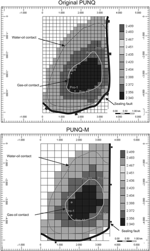
We designed a modified coarser-grid PUNQ-M (top map shown in bottom part of ), in which each permeability/porosity of this new model was obtained by calculating the arithmetic mean of four grid adjacent blocks from the original PUNQ model. Thus, PUNQ-M has a 10 × 14 × 5 grid, with 488 of those being actives. Hereafter, we will always refer to the PUNQ-M, unless otherwise stated. Each block has approximately 360 m length and total thickness of approximately 155 m. All other model input parameters from the original PUNQ model were kept the same.
The modification described allowed us to tackle the problem using a simple PC because COMPLEX is a relatively CPU-time consuming method. Nonetheless, the resulting history match problem () still has the fundamental aspects of a real-scale problem (large number of unknowns and large variability of the solutions). We used PUNQ-M to demonstrate that the combined usage of smoothness constraint and statistics on a set of quasi-solutions can produce both stable and geologically meaningful estimates. We are confident that keeping the original PUNQ number of unknowns is a mere computational power issue rather than a matter of methodology.
PUNQ-M has six production wells and is structurally controlled by a sealing fault in the east and south directions (), imposing a Dirichilet condition on these boundary segments; towards the west and north, there is an aquifer maintaining the pressure and avoiding the need of injection wells. The block initial pressures are determined from the hydrostatic equation and saturations from capillary pressure tables Citation5, Citation6. Each block saturation value is assigned as the saturation prevailing at the block centre and the initialisation conditions for the gravity–capillary equilibrium are performed for a reservoir containing water, oil, and gas phases. The depths of the gas–oil and water–oil contacts are 2355 and 2395 m, respectively Citation5, Citation6.
Here, our goal is to history match 16.5 years of production (BHP, GOR and WCUT observations) provided by the PUNQ-M reservoir by inverting the horizontal permeability (kh) and the porosity field (φ). Each model contains 488 values of kh and 488 values of φ.
Zero-mean Gaussian noise was added to the synthetic production data of the PUNQ-M values in order to simulate ‘observed’ real data. The SD of the noises are: (i) 100 Pa (Pascal) for shut-in BHPs and 300 Pa for flowing BHPs; (ii) 10% of the actual value for GORs is less than 90 and 25% of the actual value for GORs is greater than 90 and (iii) the greater of 25% of the actual value or 0.02 for WCUTs Citation5. Please note that the noise level is considerably high and mimics the actual measurements of a producing hydrocarbon field.
5. Permeability and porosity field estimation using the smoothness constraint
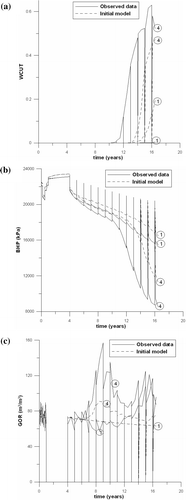
We now present results for the inversion of kh and φ fields using the smoothness constraint. To initiate COMPLEX method, the initial point is an uniform model both for kh and φ obtained by assigning for each layer the arithmetic average of the values of kh and φ in that layers, found in the well blocks of PUNQ-M. As shown in , the initial point provides a very poor match of the ‘observed’ data. This is a rather pessimistic initial point because the initial model could be better set up by krigging the values of kh and φ known at the wells.
Figure 2. WCUT (a), BHP (b) and GOR (c) produced by the initial point used in COMPLEX method, shown in dashed line, for wells Pro-1 and Pro-4 indicated by numbers inside circles. In the same figures, observed data (noise-added PUNQ-M production data) are shown in continuous line.
The role of λglb in equation (4) is to reduce the variation of kh and φ along the same layer of the reservoir. Here, we are not assuming smoothness in the vertical direction. This is a very plausible assumption, since that a depositional pulse may not be related to the previous one. In other words, only the continuity of the lateral distribution of sands in a channel is preserved.
shows the impact of increasing λglb in the variability of the solutions achieved by the COMPLEX algorithm at the end of the iterative process. Each point in represents the average of the SD of φ (left-hand side) and kh (right-hand side) for the entire set of quasi-solutions. So, we are quantifying the entire reservoir model variance in a practical way (in fact one can do this for any real reservoir). As expected, when λglb increases, the variability of the model parameters decreases. The error bars in the is ±1 SD of this average; they also decrease with increasing λglb.
Figure 3. Porosity (φ) and horizontal permeability (kh) SD averages (black circles) and their respective SD (error bars) calculated from the entire set of quasi-solutions obtained with the COMPLEX method as function of λglb. Absolute permeability values are in milidarcy.
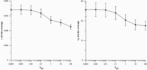
It is interesting to notice that present the same fall-off around λglb = 10−2–fact 1, nonetheless the size of the error bars decrease in different rates for φ (left side) and kh (right side)–fact 2. Besides, the decrease in the size of the error bar for φ is greater than for kh–fact 3. All three facts reveal that the normalisation factors are being correctly applied (equations (4–8)) and that the inversion is more sensitive to porosity than to the permeability logarithm. In other words, as expected, a variation of, for instance, 25% in the porosity has more impact than the same variation in log kh.
The sudden drop on the average variability is an indicator that has been tuned. At the value of λglb = 10−2 we should have attained the optimum trade-off between bias and stability of the solutions Citation14, Citation15.
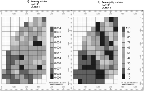
Another way of looking to the effect of increasing λglb is shown in and . In , the SD for every reservoir model parameter estimate (kh and φ) for layer 1 are shown. For λglb = 10−4 (small value of λglb), the effect of the constraint is unnoticeable and we get a rather large variability in the quasi-solutions. shows a very different behaviour: when λglb is larger, 102, the variability in the solutions is reduced and the resulted average obtained from the set of quasi-solutions for kh and φ field exhibits a very small spatial variability, resulting in an unrealistic reservoir model.
Figure 4. (a) Porosity (φ) and (b) horizontal permeability (kh) SD maps for layer 1 of PUNQ-M, calculated from the entire set of quasi-solutions obtained with the COMPLEX method using λglb = 10−4. Absolute permeability values are in milidarcy.
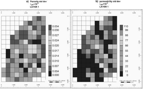
Figure 5. (a) Porosity (φ) and (b) horizontal permeability (kh) SD maps for layer 1 of PUNQ-M, calculated from the entire set of quasi-solutions obtained with the COMPLEX method using λglb = 102. Absolute permeability values are in milidarcy.
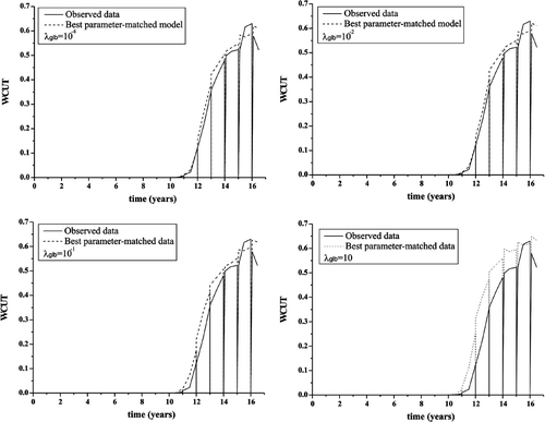
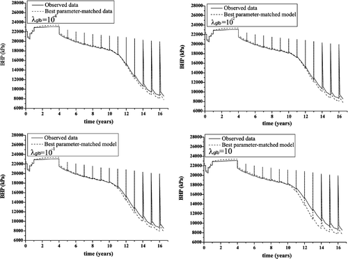
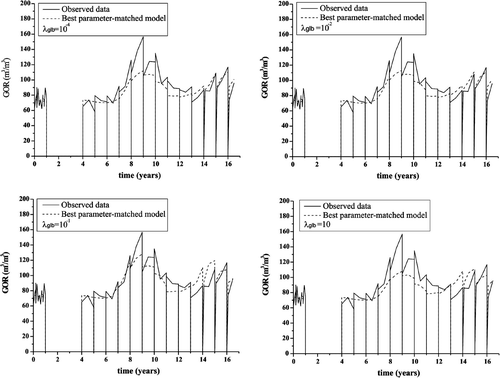
Figures show the history match curves respectively for WCUT, BHP and GOR for producer Pro-4 with λglb varying from 10−4 to 10. Despite a slight degradation of the fitting with increasing λglb, matches are fairly similar; this is an indication that there is an inherent equivalence in the solutions. However, judging from the analysis in and , the value of = 10−2 is chosen because it has the smallest bias from the constraint still providing a good fit on the observation.
We stress that was tuned without the a priori knowledge of the truth model. However, we need a measure of the parameter variability in order to tune
. Here, resides the advantage of using a method, like COMPLEX, which provides a set of quasi-solutions from where statistics can be produced.
In the case of a real history match procedure, the reservoir engineer can also judge the quality of the solutions from the match of the production curves and the geological appearance of the inverted reservoir model parameters.
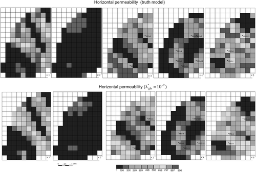
Just for comparison purposes, we show in and the truth model and the best quasi-solution of φ and kh fields for all reservoir model layers using the value of as 10−2. We were able to reconstruct both the permeability/porosity field and honour the observations. In layers 2 and 4, where the permeability and porosity of the truth model is smoother, the results of the inversion are in remarkable agreement with the truth model. For the other layers, the resemblance is also very good. For example, note that we are actually able to reconstruct very well the channel directions and fairly well their widths.
Figure 9. Upper panel: truth porosity fields for the five layers of PUNQ-M. Lower panel: porosity fields obtained from the COMPLEX point having the smallest value of Q (equation (4)) for the corresponding layers in the upper panel. It was used = 10−2.
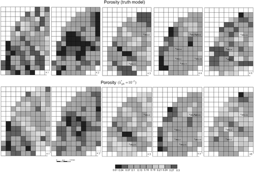
Figure 10. Upper panel: truth horizontal permeability fields for the five layers of PUNQ-M. Lower panel: horizontal permeability fields obtained from the COMPLEX point having the smallest value of Q (equation (4)) for the corresponding layers in the upper panel. It was used = 10−2. Absolute permeability values are in milidarcy.
It is very worth noticing that the obtained value of = 10−2 is very close to others found using very simple synthetic reservoir models according to our personal experience. That suggests a ‘low non-linearity’ of the associated inverse problem.
Finally, the added noise content is representative of real data Citation5. If the noise level is somewhat greater, there is less resolution in the data and, as consequence the value for would be comparatively higher. In any case, the methodology employed here to tune the
would be the same.
6. Conclusion
History match is of paramount importance on the characterisation of a reservoir and to forecast its performance. Usually, the history match procedure requires the minimisation of a function that measures the misfit between the observed and simulated data obtained from a reservoir simulation. The simulated data are usually obtained by modifying the reservoir model parameters at each iteration; this iteration stops when the difference between the observations and simulated data are small. However, because of the inherent non-uniqueness and instability of the inverse problem associated to the history match procedure, there is no guarantee that the set of parameters producing a good fit to the observations corresponds to the geological reality of the reservoir model parameters (and might not be a good representation of the geological reality) despite the model parameters could lead to a very good fitting of the observed data. Attempts to the reduction of the ambiguity may be the inclusion of constraints.
We believe that an important source of solution ambiguity is our inability to convert complex qualitative geological reality into a mathematical formulation that can be included in the objective function. In this article, we used a reservoir model based in the well-known PUNQ model. Our goal here was to history match 16.5 years of production by minimising an objective function that takes into account both the data misfit and the geological information. Here, the geological constraint in the objective function is the smoothness constraint over the entire set of horizontal permeability and porosity fields: the constraint requires that the spatial variation of the parameters to be inverted have minimal variance. However, since we never have guarantee that the constraint used reflects the geological reality, we must use the smallest amount of this constraint in the minimisation of the objective function.
We showed that the right use of the smoothness constraint reduces the ambiguity, introduces minimum bias in the inverted model parameters and produces good fit between the observations and the simulated results. The tuning of the right/optimum value of the parameter controlling the degree of smoothness is found without the knowledge of the truth model and in a practical approach that may be applied to a real reservoir. The remarkable agreement of the amount of smoothness required to stabilise the solution with this example and with other synthetic models lead us to suggest that the associated inverse problem may have a small degree of non-linearity.
We are aware that smoothness constraints cannot be employed in all reservoirs. However, we believe that when the appropriate geological constraint is applied in a given problem, it will help to evaluate the uncertainty in the reservoir model parameters and therefore in the production forecast. In other words, we trust that a tool box for the HM problem can be designed. Each tool incorporates a different constraint, so that the interpreter can judiciously choose the most suitable tool to help on a specific HM problem.
Acknowledgements
The authors wish to thank ‘Rede Cooperativa de Pesquisa–Caracterização Geológica e Geofísica de Campus Maduros’ (FINEP/CTPETRO/PETROBRAS) for financial support. FLS thanks CNPq for his MSc scholarship. AFdN and WEM thank CNPq for their research grants. All the fluid flow simulations were done using IMEX® from CMG Ltd. Finally, we thank the Associated Editor, Prof. Anatoly G. Yagola and three anonymous reviewers for improving the original manuscript.
References
- Wu, Z, Reynolds, AC, and Oliver, DS, 1998. Conditioning geostatistical models to two-phase production data, Paper SPE 49003 presented at the 1998 SPE Annual Technical Conference and Exhibition. New Orleans. 1998.
- Mantica, S, Cominelli, A, and Mantica, G, 2001. "Combining global and local optimization techniques for automatic history matching production and seismic data, 2001". In: Paper SPE66355 presented at the 2001 SPE Reservoir Symposium Simulation. Houston, TX. 2001.
- Tavassoli, Z, Carter, JN, and King, P, 2004. Errors in history matching, SPE Journal (2004), pp. 352–361.
- Tikhonov, AN, and Arsenin, VY, 1977. Solutions of Ill-Posed Problems. New York: John Wiley & Sons; 1977.
- Barker, JW, Cuypers, M, and Holden, L, 2001. Quantifying uncertainty in production forecasts: another look at the PUNQ-S3 problem, SPEJ (2001), pp. 433–441.
- Floris, FJT, Bush, MD, Cuypers, M, Roggero, F, and Syversveen, A-R, 2001. Methods for quantifying the uncertainty of production forecasts: a comparative study, Petroleum Geoscience 7 (2001), pp. S87–S96.
- Richardson, JA, and Kuester, JL, 1973. The complex method for constrained optimization, Communications of the ACM 6 (1973), pp. 487–489.
- Peaceman, DW, 1977. Fundamentals of Numerical Reservoir Simulation. Amsterdam: Elsevier Science Publishing Company; 1977.
- Thomas, GW, 1982. Principles of Hydrocarbon Reservoir Simulation. Boston: International Human Resource Development Corporation; 1982.
- Silva, JBC, Medeiros, WE, and Barbosa, VCF, 2001. Pitfalls in nonlinear inversion, Pure and Applied Geophysics 158 (2001), pp. 945–964.
- Silva, JBC, Medeiros, WE, and Barbosa, VCF, 2001. Potential field inversion: choosing the appropriate tecnhique to solve a geologic problem, Geophysics 66 (2001), pp. 511–520.
- Brun, B, Gosselin, O, and Barker, JW, 2001. Use of prior information in gradient-based history-matching, Paper SPE 66353 presented at the 2001 SPE Reservoir Symposium Simulation. Houston, TX. 2001.
- Medeiros, WE, and Silva, JBC, 1996. Geophysical inversion using approximate equality constraints, Geophysics 61 (1996), pp. 1678–1688.
- Parker, RL, 1977. Understanding inverse theory, Annual Review of Earth Planetary Sciences 5 (1977), pp. 35–64.
- Menke, W, 1984. Geophysical Data Analysis: Discrete Inverse Theory. New York: Academic Press; 1984.
