Regularized solution of the solar Bremsstrahlung inverse problem: model dependence and implementation issues

Abstract

We address an important inverse problem in solar plasma physics by means of an ‘ad hoc’ implementation of the Tikhonov regularization method. Our approach is validated in the case of different modifications of the mathematical model of the problem based on physical motivations, and for data sets obtained with synthetic experiments. Finally, an application to a real observation recorded by the NASA mission ‘Reuven Ramaty High Energy Solar Spectroscopic Imager (RHESSI)’ is considered.

Keywords:

• Inverse problems
• Solar flares
• Regularization theory

1. Introduction

Solar flares 1–3 are the most dramatic and mysterious events in the solar system. These transient phenomena are characterized by a sudden release of huge amounts of energy of magnetic origin and are revealed by electromagnetic emission mostly in the X-ray energy range. Particularly intense events may release up to 10³³ ergs in a few seconds and accelerate electrons in the solar plasma with a rate up to 10³⁷ per second. This means that the electrical currents passing through the solar chromosphere during a flare have orders of magnitude of around 10¹⁸ ampère, corresponding to magnetic fields of around 10⁴ tesla. The main theoretical problem with solar flares is that no mathematical modelization so far formulated (based on the well-established equations of plasma physics and magnetohydrodynamics) is able to fully explain such remarkably large numbers. Most physical interpretations of X-ray emission during solar flares are based on the assumption that a collisional interaction takes place between accelerated electrons and steady ions in the plasma. During such phenomenon, named Bremsstrahlung collision 4, light charged particles (electrons in this case) are deflected and slowed down by the presence of other heavier charged particles (the ions in the solar chromosphere) and loose their energy in form of electromagnetic radiation mainly at X-ray wavelengths. Several solar missions have been designed with the aim of detecting such radiation. For example, the on-orbit solar satellite Yohkoh, launched in August 1991, was able to collect radiation from electronic collisions in the case of both soft (energies in the range 0.25–4 keV) and hard X-rays (energies up to nearly 100 keV). The Reuven Ramaty High Energy Solar Spectroscopic Imager (RHESSI) 5, launched by NASA on February 2002, is currently recording hard X-rays and γ-rays up to 1 MeV during solar flares.

From a mathematical viewpoint, Bremsstrahlung collision is fully described by a quantity, named Bremsstrahlung cross-section, which represents the probability that a hard X-ray photon of given energy is produced by an electron in the plasma of given (bigger) energy. Therefore, the mathematical description of solar Bremsstrahlung is based on a Volterra integral equation, from now on named the Bremsstrahlung equation, which relates the emitted photon spectrum with the flux spectrum of the electrons in the source and where the integral kernel is represented by the Bremsstrahlung cross-section. The importance of the exciting electron flux spectrum in this theory relies on the fact that its determination from the observed X-rays depends only on the Bremsstrahlung cross-section and does not require any modelling assumption on the acceleration or propagation mechanisms 6. Furthermore the Bremsstrahlung equation can be easily generalized to account for second order phenomena like albedo 7 or anisotropies in the emission direction 8.

The study of the inverse problem of determining the electron flux spectrum from measurements of the emitted photon flux has been accomplished in several papers from the astronomical community. In particular, in 9 the formulation of the solar Bremsstrahlung problem in terms of a Volterra integral equation of the first kind is introduced for the first time together with an analytical approach to its solution. The ill-posedness of the problem is pointed out in 10 and re-construction approaches for its solution are discussed and validated in 10–15. Finally in 6 some theoretical implications of this formulation of the problem are derived together with some hints on the physical interpretation of re-constructed electron spectra.

The contribution of the present article to this investigation is 2-fold. First we will study the sensitivity of the inverse problem solution to the modification of the integral kernel due to different assumptions on the Bremsstrahlung cross-section. Indeed nuclear physics provides several possible different forms for the Bremsstrahlung cross-section, depending, for example, if relativistic or Coulomb corrections are included in the modelling. Some of these forms are easy expressions and in these cases some analytical results can be obtained from the study of the corresponding Bremsstrahlung integral equation. However more general and reliable forms for the cross-section are extremely complicated functions of the photon and electron energies and for them only numerical investigations are reasonably possible. Our study will be based on both a singular value decomposition analysis of the Bremsstrahlung equation and a regularized inversion of the X-ray data based on the Tikhonov method 16.

The second issue we will address is to describe the mathematical content of an inversion code for the analysis of RHESSI data the authors of the present article have implemented and which has been included in the software of the satellite mission. Although this code accomplishes such analysis by means of the classical Tikhonov approach, here we discuss some specific procedures which have been utilized in the implementation, for determining the error and resolution bars, for choosing the optimal value of the regularization parameter and for handling the notable dynamical range typical of RHESSI data.

The plan of the article is as follows. Section 2 will perform the mathematical setup of the problem and contain the definition of all the quantities we will use in the equations. Section 3 will provide some analytical results in the case of two possible approximations of the Bremsstrahlung cross-section. In section 4 a first analysis of the consequences of changes in the integral kernel of the Bremsstrahlung equation will be addressed by means of a singular value decomposition approach. Section 5 contains a description of the inversion software implemented for the RHESSI mission and gives particular emphasis on the issues of choosing the regularization parameter and re-scaling the dynamical range of the input data. In section 6 the regularized inversion of the Bremsstrahlung equation is performed in the case of both significant simulated data and a real spectrum measured by RHESSI. This section will consider effects of variations in the integral kernel by comparing regularized solutions corresponding to different cross-sections. Our conclusions will be offered in section 7.

2. The Bremsstrahlung equation

Following 9 and 6, we first define the mean target proton density in the source as (1) and the mean electron spectrum (2) where V is the source volume, n(r) is the local proton density in the plasma and F(E, r) is the local electron distribution function. Then the photon spectrum I(ε) observed at distance R from a source, measured in photons cm⁻² s⁻¹ keV⁻¹, is given by (3) where Q(ε,E) is the Bremsstrahlung cross-section, which is a function of both the photon energy ε and the electron energy E. If we define (4) equation (3) becomes (5) Equation (5) is the Bremsstrahlung equation in solar plasma physics: it can be written without any prescription or assumption on the physical processes in the source and just for this reason it is the most general equation describing the X-ray emission mechanism during solar flares. We point out that this model is completely isotropic, i.e. no angular dependency in the mean electron spectrum or in the cross-section is considered, and, furthermore, that secondary effects like albedo are not taken into account. First investigations toward anisotropic modellization of the emission or interpretations of the re-constructed f(E) which involve albedo have been described in 8 and 7, although further generalizations of equation (5) are in progress.

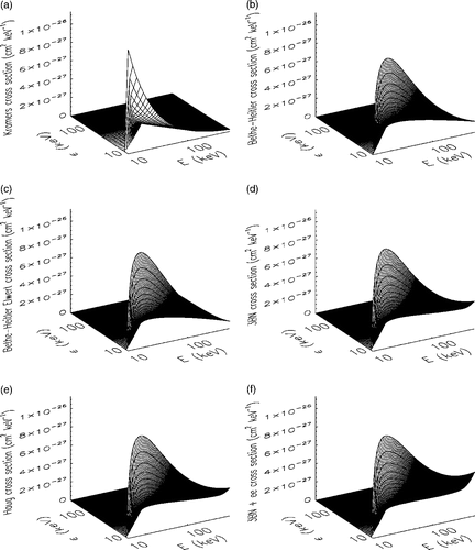
A crucial role in equation (5) is played by the cross-section Q(ε, E). Indeed, this function carries a significant physical meaning, describing the effectiveness of the Bremsstrahlung process. On the mathematical side, its analytical shape has important consequences on the numerical stability of the solution process and represents a reliable indication of the information content which can be retrieved from the X-ray data. According to the physical conditions where the emission process takes place, many different forms of such a cross-section can be written 17. Here we consider six possible forms (which are among the most utilized in solar physics) and, for sake of simplicity, group them in two families.

Family I:

It contains two cross-sections which have a simple analytic expression and, physically, are non- and mildly-relativistic, respectively. The two cross-sections are the Kramers (K) cross-section 18 (figure 1(a)) (6) and the Bethe–Heitler (BH) cross-section 17 (figure 1(b)) (7) Q₀ is (8) where Z is the atomic number of the target, m and r₀ are the mass and the classical radius of the electron and c is the speed of light.

Figure 1. The six cross-sections considered in the article: (a) Kramers cross-section (formula K in the text); (b) Bethe–Heitler cross-section (formula BH in the text); (c) Bethe-Heitler cross-section with Elwert correction for Coulomb effects (formula BHE in the text); (d) 3BN cross-section with highly relativistic effects (formula 3BN in the text); (e) Haug interpolated cross-section (formula H in the text); (f) 3BN cross-section with electron-electron interaction effects (formula 3BNee in the text).

Family II:

It contains four cross-sections which include physical second order effects. Analytically all forms are extremely complicated and therefore will not be reported here (but appropriate references to papers where these forms can be found are given). In particular, the Bethe–Heitler–Elwert (BHE) cross-section 12 (figure 1c) modifies the Bethe–Heitler formula (7) to account for Coulomb effects at low energies. The 3BN cross-section 17 (figure 1d) includes all relativistic effects. The Haug (H) cross-section 19 (figure 1e) is obtained by interpolating the 3BN formula and its computation is less expensive. Finally, the 3BNee cross-section 20 (figure 1f) is a correction of the 3BN formula which accounts for the electron-electron interaction significant at high energies.

There are essentially two reasons why it is interesting to study equation (5) for different forms of the cross-section. The first one is physical and is the fact that the differences in the solution f(E) for the different forms of Q(ε, E) previously introduced can provide quantitative information on the incidence of the relativistic, Coulomb, electron–electron interaction corrections on the photon production in the solar plasma. The second reason is computational and is the fact that the numerical solution of equation (5) is notably less onerous in the case of equations (6)–(7) and then it is helpful to verify whether (and to what extent) the second order effects can be neglected in the solution procedure.

3. Analytical results

In this section, we present some analytical results concerned with equation (5) obtained when the integral kernels are cross-sections K and BH in equation (6) and (7), respectively. For these kernels, equation (5) can be analytically solved by applying the theory of Mellin transform 21. The Mellin transform of a function f : (0, ∞) → ℝ such that for some real number σ in (0, 1/2), is defined as (9) with ξ ∈ (−∞, ∞). The corresponding inversion formula is (10) In the case of linear integral equations of the first kind, when the kernel depends on the variables ratio, i.e. (11) the Mellin transform applied to both sides leads to the diagonalization (12) For cross-sections K and BH, the Bremsstrahlung equation (5) assumes the same form as in (11). In fact, if one introduces the new integral kernel (13) and defines the new data function (14) equation (5) becomes (15) where (16) for formula K and (17) for formula BH. Therefore the following theorem holds:

Theorem 3.1

The analytical form of the solution of equation (5) is given by (18) in the case of cross-section K and by (19) in the case of cross-section BH.

Proof

Let us introduce the Beta Function B(p, q) defined as (20) and the relation B(p,q) = (Γ(p)Γ(q)/Γ(p + q)) between this function and the Gamma Function (21) Therefore, for case K, (22) For case BH, integration by parts leads to (23) where v(x) is defined as (24) Since (25) and we have (26) ▪

Equations (22) and (26) show that both and are entire functions which tend to zero continuously for |ξ| → ∞. This implies that the two analytical solutions (18) and (19) do not depend continuously on the data J(ε).

In real observations the photon energies involved in the flare process belong to a bounded interval (ε_min, ε_max). Therefore a more realistic model for the Bremsstrahlung emission is given by the linear inverse problem (27) with A₁ : L²(ε_min, ∞) → L²(ε_min, ε_max) the linear operator defined as (28)

Theorem 3.2

When the integral kernel is given by formula K or formula BH the operator (28) is compact.

Proof

Let us consider first the case of cross-section K; we have to show that the function belongs to L²([ε_min, ε_max] × [ε_min, ∞]). We have and therefore the operator A₁ is Hilbert–Schmidt.

In the case of the Bethe–Heitler cross section, we make the usual change of variable x = ε/E and we have and therefore even in this case the operator A₁ is Hilbert-Schmidt.▪

Theorem 3.2 implies that the linear inverse problem (27) is ill-posed in the sense of Hadamard and therefore that even in this case the solution does not depend continuously on the data. Real measurements provide sampled values of the photon spectrum at a finite number of photon energies. In 10 the problem (29) is addressed when Q(ε, E) is the BH cross-section, by maintaining f in L²(ε_min, ∞). This approach is realistically possible only when the cross-section has a relatively simple form. In the present article we want to consider very general forms of Q(ε, E) and therefore the discretization of the Bremsstrahlung equation becomes a necessary preliminary step for inversion. However the impact of ill-posedness on the discretized equation is notable, since any discretization of equation (27) must account for the numerical instabilities due to the presence of noise on the observed spectrum.

4. Singular systems

The kind of data that real observations put at disposal of the mathematical analysis are vectors g whose components are the sampled values of the observed spectrum at N discrete photon energies ε₁, …, ε_N, i.e. (30) We choose as data space the finite dimensional vector space Y equipped with the inner product (31) where the w_ln (l, n = 1, …, N) are appropriate weights depending on the energy sampling. The discretized inverse problem we have to solve in practice is therefore the linear system (32) where f is the solution vector with components (33) E₁, …, E_M are the discretized electron energies. We assume that the solution space X is the canonical ℝ^M. A is the rectangular matrix with entries (34) η_nm being the quadrature coefficients. For reasons related to the physics of the problem and, in particular, to the characteristics of the acquisition procedure applied by RHESSI, in the following we will always assume M > N. Of course the explicit form of the entries (34) will be different for the six different possible choices of the cross-section.

The generalized solution of the linear system (32), i.e. the vector solving the constrained least-squares problem (35) is (36) where p is the rank of the matrix A and is its singular system defined as (37) Problem (35) is well-posed in the sense of Hadamard but, owing to the ill-posedness of the original continuous problem (27), it is ill-conditioned. The dependence of the degree of ill-conditioning with respect to the cross-section can be quantitatively assessed by means of the singular system of the matrix A when the six different formulas for the integral kernel Q(ε, E) are adopted. The setup of this numerical experiment is as follows. We consider N = 240 photon energies from ε₁ = 10 keV to ε_N = 249 keV, with a uniform sampling distance of 1 keV. The electron energies are M = 480, from E₁ = 10 keV to E_M = 489 keV and are again uniformly sampled with 1 keV binning (these choices are realistic in the framework of typical RHESSI observations). Therefore both the weights in the vector data space and the quadrature weights in (34) are constant and equal to 1. In figure 2 we plot the normalized singular spectra corresponding to all six cross-sections, where the normalization is performed by dividing all singular values of each matrix by the first one. In particular figure 2(a) contains the first 100 singular values corresponding to formulas K and BH, while figure 2(b) contains the first 100 singular values corresponding to formulas BHE, 3BN, H and 3BNee. The general trend of these singular spectra shows that the introduction of relativistic corrections in the integral kernels increases the ill-conditioning of the problem: indeed the singular spectra corresponding to the non-relativistic and mildly-relativistic cross-sections K and BH decrease more slowly with the singular value order than in the case of the other four cross-sections. In particular, the matrix A corresponding to cross-section K is the most well-conditioned one, in accordance with the fact that Q_K(ε, E) in (6) is less smooth than the other cross-section forms (figure 1). From figure 2(b) we point out that the singular spectrum corresponding to formula H cannot be distinguished from the singular spectrum corresponding to formula 3BN, in accordance with the fact that formula H is an accurate interpolation of formula 3BN. Moreover, the electron–electron correction (accounted for in formula 3BNee) reflects into a slight increase of the ill-conditioning of the problem. Figure 3 shows the first three singular functions for each integral kernel used in the computation. A general feature for all cases is that the number of zeros increases with the order of the singular function. More in particular, we have that: the singular functions corresponding to the integral kernel K present the fastest oscillations; formulas H and 3BN provide essentially the same singular functions; the differences due to the use of formula BHE are more significant at small E.

Figure 2. Singular spectra for the six (discretized) integral kernels: (a) formulas K and BH; (b) formulas BHE, 3BN, H and 3BNee.

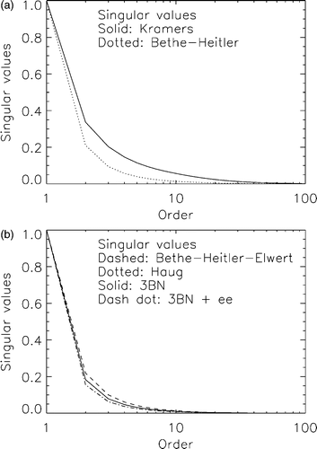
Figure 3. The first three singular functions for the six (discretized) integral kernels: (a) u₁(E) for formulas K and BH; (b) u₁(E) for formulas BHE, 3BN, H and 3BNee; (c) u₂(E) for formulas K and BH; (d) u₂(E) for formulas BHE, 3BN, H and 3BNee; (e) u₃(E) for formulas K and BH; (f) u₃(E) for formulas BHE, 3BN, H and 3BNee.

5. Inversion method

‘SolarSoftWare’ (SSW) is the IDL package officially used for the analysis of RHESSI data. Within this software, 19 routines have been implemented by the authors of the present article for the regularized inversion of photon flux spectra emitted in correspondence with flare events observed by RHESSI. In order to describe the mathematical basis of this set of routines we first discuss the regularized inversion of the solar Bremsstrahlung problem in a continuous setting, i.e. in the case of (38) where A is the integral operator defined at the right hand side of (5).

Regularization theory 22–26 is certainly the most effective tool for the solution of such a linear ill-posed inverse problem. In this framework a stable and reliable approximate solution is obtained by exploiting a priori information on both the source function f and the noise affecting the data g. However, there exist several different regularization methods and in order to choose the best approach for the present problem it is necessary to account for its mathematical and physical properties. In particular:

•	Tikhonov-like methods 16,27 look for the one-parameter family of solutions of the minimum problem (39) where X and Y are Hilbert spaces and C is a closed operator in X. The only a priori information on f available from physical considerations is that f is always positive and characterized by a huge dynamical range (five or six orders of magnitude of the electron flux can be covered within one order of magnitude in the energy E axis). At low energies, a possibly strong thermal component may induce the presence of a non-monotonic behaviour while short-wavelengths features (related, by instance, to pile-up corrections) are possible at intermediate energies. Therefore in general utilizing f ′ or even f ″ in the penalty term (i.e. utilizing the first or second derivative for C) may result in loosing these details. On the other hand, the choice C = I realizes the search for the solution of minimal energy compatible with the data, which is a physically sound condition. Furthermore, the supports of physically realistic electron flux spectra are certainly too wide for the application of a support constraint to be advantageous. This implies that the choices X = L2(εmin, ∞), Y = L2(εmin, εmax) and C equal to the identity operator are probably the most reliable.
•	Deterministic iterative approaches like the Landweber method 22 present the advantage that the positivity constraint can be rather easily implemented into the algorithm 28. However such approaches are typically computationally expensive and preconditioned versions of the schemes sometimes do not preserve a satisfactory re-construction accuracy 29.
•	A priori knowledge on the statistical properties of the noise can be exploited by iterative schemes of the Expectation–Maximization family 30. These methods have been formulated in the case of Poisson noise 31 and generalized to Gaussian noise 32,33. However the aim of our code is the analysis of X-ray spectra recorded by RHESSI and in this mission the noise affecting the measurements is not purely Poissonian, but has a systematic component of difficult modelling.

Given the previous items, our approach to the regularized solution of the solar Bremsstrahlung inverse problem has been based on Tikhonov regularization with X = L²(ε_min, ∞), Y = L²(ε_min, ε_max) and C the identity operator (anyway, the behaviour of first-order Tikhonov regularization, i.e. when C is the first derivative, has been tested in 13 while the effect of Landweber iterations with positivity constraint has been studied in the case of the Bremsstrahlung problem under thermal conditions in 34). In particular, in a discretized setting, our routines address the minimum problem (40) where the regularization parameter λ is real and positive. By using a classical variational approach and the singular system of A, it is straightforward to show that the solution of (40) is (41) We point out that equation (41) does not necessarily provide a positive solution. In order to realize the positivity condition in Tikhonov regularization a box constraint should be applied within the optimization procedure (40), which, nevertheless, would notably slow down the computation. However, in our problem, many experiments with both real and synthetic data have shown that the Tikhonov functions (41) are always positive, in accordance with the physics of the problem.

Three main issues are involved with the actual computation of formula (41): (1) the determination of an optimal value of the regularization parameter; (2) the assessment of the propagation error from the data to the regularized solution; (3) the assessment of the spectral resolution associated with the regularized solution, i.e. the size of the electron energy range whereby f presents detectable features (once the optimal value of the regularization parameter has been fixed). In the following we will describe how these issues have been addressed in our inversion software. Then, in the final part of this section, we will describe a re-scaling procedure we have adopted in order to reduce the effects of the huge dynamical range of RHESSI data onto the regularization process.

5.1. Choice of the regularization parameter

The optimal choice of the regularization parameter realizes the perfect trade-off between the complexity of the solution and its ability to reliably reproduce the experimental data. In current literature many criteria exist for addressing this optimality problem 35 and a useful hint for validating them would be to formulate a statistical test quantitatively assessing the over- or under-smoothing properties of the selected λ. For the particular case of the Bremsstrahlung inverse problem several applications 10,36 have shown that Morozov discrepancy principle 37 has often oversmoothing properties, while Generalized Cross Validation (GCV) 38 has often undersmoothing properties (these trends are confirmed for other applications 22). In order to control the smoothing properties of the selection algorithm we have applied a new approach where the optimal choice of λ is accomplished by a statistical analysis of the regularized cumulative residuals for problem (32) 15. In a stochastic framework, the data and the solution of (32) are random variables and the model (42) for the observed data can be assumed, where δg is the random variable representing the noise on the data. For each sampled photon energy ε_k we define the normalized residuals (43) The set of the cumulative normalized residuals is defined as (44) From a statistical viewpoint the normalized residuals must be consistent with the distribution of the (normalized) noise and therefore are approximately distributed according to a Gaussian function of zero mean and standard deviation equal to 1. It follows that the sum represents a random walk whose variance is j and therefore c_j has standard deviation . When the regularization switch is on, i.e. if λ ≠ 0, we can introduce the regularized normalized residuals (45) and the regularized cumulative normalized residuals (46) Now the sum is not a random walk (here also the regularized solution f_λ is considered as a random variable). However, if λ is fixed in such a way that a specific realization of is in the range for all j, then such realization can be considered as one of the realizations of c_j oscillating in this range with a probability larger than 99%. This suggests that the comparison between as a function of j and the bounds can be considered a reliable statistical test to evaluate the under- or over-smoothing effects of the optimally selected λ. And, even more, a heuristical regularization algorithm can be formulated on the basis of this statistical test. In fact, if, by instance, the selection criterion adopted provides an oversmoothing value for λ, i.e. if for some j, then λ can be decreased up to the maximum value where (47) (when the choice criterion is undersmoothing the λ value should be increased up to the maximum value where (47) is verified). In our code this heuristic procedure is used to tune the value of the regularization parameter provided by the discrepancy principle 37. We finally point out that several stochastically-based criteria for the choice of the regularization parameter have been recently introduced in the literature for both linear and non-linear ill-posed problems (see, for example, 39,40). The main characteristics of our semi-heuristic approach are that, first of all, its implementation is straightforward since it simply requires a comparison between the experimental and the regularized residuals. Furthermore, the method is quite general, since for its application it is not necessary to introduce strict hypothesis on the statistical properties of the noise distribution or to a priori know overall bounds on the noise amount (we use the discrepancy principle only as an initialization but any other initial guess can be applied in order to initialize the iteration on λ).

5.2. Errors and resolution bars

The determination of the propagation error on the regularized solution is performed by means of the computation of the confidence strip 27. Many different random realizations of the input photon spectrum are realized and the corresponding regularized solutions are superimposed to determine a strip of re-constructed electron flux spectra all with the same regularization parameter determined by means of the heuristic approach described in the previous section. The width of the confidence strip provides the error bar on the regularized solution at each sampled electron energy.

In order to assess the spectral resolution, we have already observed in section 4 that the singular vectors u_k are characterized by a number of oscillations around zero which increases with their order. On the other hand, the regularization parameter damps the contribution of high order singular components so that only a few of them are really effective in the re-construction of the electron spectrum. In order to determine the last significant singular component in the expansion (41) we introduce the power spectra P₁ and P₂ of f and δ_g, respectively defined as (48) and (49) where ⟨·,·⟩ denotes the average over all possible data realizations. From equations (42) and (37) we easily obtain the relation (50) The crucial point in equation (50) is that the first term at the rhs, i.e. the signal component, decreases with k while the second one, i.e. the noise component, is constant. In particular, the signal part stays larger than the noise part until (51) Now P₂/P₁ is not explicitly known in general but regularization theory assures that is a reliable estimate of this ratio, so that the truncation condition 27 (52) for the expansion (41) is reasonable. Therefore, if is the first singular value satisfying (52), a measure of the resolution limit achievable by Tikhonov method is given by the distance between two successive zeros of the corresponding last significant singular vector . Since in our implementation the electron energies are discretized before the inversion, the software provides, as resolution limit, the distance between the two sampled electron energies closest to the successive zeros.

5.3. Re-scaling

A peculiar feature of solar photon spectra is its huge dynamical range: for a photon energy range between 10 keV and 100 keV the most energetic flares present photon fluxes which decrease from around 10⁵ to 1 photons cm⁻² keV⁻¹ s⁻¹. From the viewpoint of regularization this implies that the estimate of the regularization parameter, which is a global parameter tuning stability and fitting over the whole energy range, may be unreliable. To overcome this difficulty, in our approach a re-scaling procedure is applied, which flattens the input photon spectrum together with a coherent modification of the electron spectrum and of the integral kernel. The idea is to re-scale the fundamental equation (5) to the form (53) with (54) and (55) Now the problem is how to optimally determine the value of the re-scaling parameter. To this aim we first observe that a typical solar photon spectrum is a slight modification of an overall double power-law behaviour (56) Hence we implemented the following computational procedure:

•	in simulation and for a single power-law g(ε) ∼ ε−γ we fixed a value of γ, applied the regularized inversion for different values of p and selected the p value for which the regularized solution best fit (according to χ2 statistics) the original data;
•	we repeated the process at the previous step for many values of γ in a realistic range and built up a look-up table which provides the optimal value of p for each γ value;
•	the number of values of the look-up table is increased by means of a spline interpolation;
•	given a real spectrum, we fit it with a double power-law, determine the fitting parameter γ1 and γ2, compute , find the closest γ in the interpolated look-up table and assign the corresponding p value.

6. Regularized re-constructions

The effectiveness of this implementation of Tikhonov regularization for solving the solar spectroscopy inverse problem is tested here in the case of both synthetic and real data. In particular, simulations are concerned with the determination of the so-called spectral index in the easiest case of a monotonically decreasing photon spectrum and with the re-construction of a realistic form of the averaged electron flux spectrum. The real case refers to the inversion of a photon spectrum recorded by RHESSI in correspondence of the solar flare occured on 3 November 2003.

6.1. Spectral index

The local spectral indices associated with a photon and an electron spectrum are defined as (57) and (58) One of the main reasons why spectral indeces are introduced in solar physics 41 is because they provide information on the X-ray emission without depending on the absolute magnitude of the event and therefore allow a quantitative comparison of flares of different size. As discussed in section 5.3, many flares produce photon spectra with overall behaviours of a power-law or double power-law and therefore are characterized by constant or piecewise constant spectral indeces. Due to equation (5) the local electron spectral index must be quantitatively related to the local photon spectral index. In the case of cross-sections K and BH integration by parts immediately shows that the electron spectral index corresponding to a constant photon spectral index γ is constant and is given by (59) However this relation is not true in general for the other integral kernels. 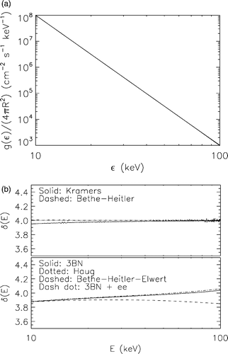In order to study how relation (59) is modified by the introduction of more complicated cross-sections we consider the photon spectrum in figure 4(a) which is obtained by affecting the function (60) with a realistic Poisson noise. The spectrum has been simulated by using 996 samples uniformly distributed in the energy range (1,200) keV. The inversion has been done by considering electron energies with the same uniform binning but over the range (1,400) keV. Tikhonov regularization method is applied for all six cross sections and the corresponding six electron spectral indeces are computed in the two panels of figure 4(b). As expected, δ(E) is very close to four when formulas K and BH are used (the deviations are due to numerical reasons and decrease if the computation precision is increased) while significant modifications from the constant values are introduced by the Elwert correction (formula BHE) and by accounting for relativistic effects (formulas 3BN and H) or effects due to electron–electron interaction (formula 3BNee).

Figure 4. Estimate of the spectral index by means of regularized inversion: (a) input photon spectrum, a power-law with constant spectral index 5; (b) re-constructed electron spectral index obtained in the case of the six cross-sections considered in the article.

6.2. Re-construction of the averaged electron flux spectrum

A realistic synthetic data set is constructed by considering first the theoretical averaged electron flux spectrum (61) where C₁ = C₂ = 5 · 10⁵, δ₁ = 4 and δ₂ = 5, represented in figure 5(a). This function presents two features which are predicted by most theoretical models for solar flare physics: a spectral ‘knee’ at intermediate energies, typically representing a signature of the slowing down of the emission at higher energies, and a Maxwellian component which becomes significant at low energies and which accounts for possible thermal emission. Then equation (61) has been inserted into equation (5) when the integral kernel is the most general cross section, i.e. formula 3BNee, and realistic Poisson noise is added for each data component. In the case of Poisson noise the relative error depends on the energy: in our simulation, it is around 0.1% at low ε and grows up to more than 30% at high energies. The result is the simulated photon flux spectrum in figure 5(b) uniformly sampled with 240 points from 10 keV to 249 keV. This vector is inverted by means of our regularization code. In order to avoid an ‘inverse crime’ procedure the inversion has been performed by using the five cross-sections different than the one utilized to produce the data in the forward procedure (namely formula 3BNee). The reconstructions are presented in figure 5(c) in the case of formulas K and BH and in figure 5(d) in the case of formulas BHE, 3BN and H. Here the electron flux spectra are uniformly sampled with 489 points from 10 keV to 498 keV. From a quantitative viewpoint the inversion outcome can be assessed by some reconstruction error whose computation is based on the comparison with the theoretical form (61). In this application, for each one of the five inversions we have computed the relative root mean square error (62) The results given in table 1 and figure 5 show that:

•	the use of the classical formulas K and BH produces the most inaccurate results;
•	formulas 3BN and H provide very similar (and accurate) re-constructions, which is reasonable, since H is an interpolation of 3BN;
•	BHE works fine at small energies but rather badly at high energies. The fact that the spectrum is very steeply decreasing explains the small re-construction error in the table for this cross-section.

Figure 5. Re-construction of a theoretical input averaged electron flux spectrum by means of regularized inversion: (a) theoretical input electron spectrum, a broken power-law with thermal component; (b) simulated photon flux spectrum; (c) regularized solutions in the case of formulas K and BH; (d) regularized solutions in the case of formulas BHE, 3BN and H.

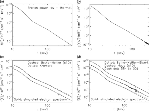
Table 1. Re-construction errors (%) in the restoration of Equation (61) in the case of five cross-sections considered in the article. Formula (62) has been used to assess the re-construction errors

Cross-section	err
K	20.7
BH	30.8
BHE	2.6
3BN	9.0
H	8.5

We have performed numerical experiments like this one for many theoretical forms of the input electron spectrum and the results are coherent with the ones in the table and in the figure.

6.3. Real data

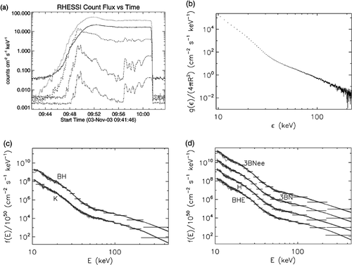
As an example of application to real data we consider the flare event recorded by RHESSI on 3 November 2003. The number of counts detected by the satellite for different energy ranges is given in figure 6(a) for the time interval 09:41:44–10:03:40 UT. The photon flux spectrum considered in the inversion has been built up by processing these counts in the time interval 09:57:00–09:57:20 UT and the resulting spectrum, uniformly sampled with 397 points from 9 keV to 223 keV, is given in figure 6(b). This data vector has been inverted by means of our code for all cross-sections to give the re-constructed electron flux spectra, uniformly sampled with 437 points from 9 keV to 446 keV, in figure 6(c) and figure 6(d). For each re-construction we give the confidence strip and the resolution bars computed as explained in section 5.2. We point out that the overall behaviour is approximately the same for all regularized solutions, which denotes a notable robustness of the inversion procedure with respect to the modification of the model. As an example of a more quantitative analysis, we computed the photon and electron spectral indeces for all cases. In the photon energy range [70, 200] keV the best fit for γ(ε) is γ ≃ 3.83; in the same range of electron energies we found that equation (59) is approximately satisfied for cross-sections K, BH, 3BN, H and 3BNee (in particular, δ ≃ 2.63 for formula K) while a more significant displacement occurs in the case of cross section BHE (δ ≃ 2.23).

Figure 6. Application to RHESSI data: (a) count flux in the case of the solar flare of 3 November 2003. The counts detected in five increasing energy channels are plotted without background removal (solid: 6–12 keV, dotted: 12–25 keV, dashed: 25–50 keV, dash dot: 50–100 keV, dash dot dot: 100–300 keV); (b) the photon flux spectrum constructed from the counts in (a); (c) reconstructed averaged electron flux spectrum for formulas K and BH; (d) reconstructed averaged electron flux spectrum for formulas BHE, 3BN, H and 3BNee.

7. Conclusions and open problems

The main content of this article was computational and aimed at discussing an implementation of Tikhonov regularization method which is ‘ad hoc’ for an important inverse problem in solar X-ray physics. The scientific motivation of this effort was the launch performed by NASA in 2002 of the solar satellite RHESSI with the precise intent of recording X-ray emissions from the Sun during flares. In particular, we discussed the incidence of changes in the cross-section, i.e., mathematically, in the integral kernel, on the regularized solution, showing that the overall behaviour of the re-constructions is preserved during the inversion but that significant differences occur if an analysis of more quantitative features like spectral indeces or slope changes is performed. From a methodological viewpoint, we believe that some issues of our implementation (like the choice criterion for the regularization parameter based on the analysis of cumulative residuals or the data re-scaling procedure) have a general potentiality and can be applied to other linear inverse problems.

Possible further applications of this approach to the Bremsstrahlung inverse problem may concern:

•	a statistical study of a large number of flares, possibly classified on the basis of their size and intensity, in order to point out general trends on the emission mechanism;
•	an application to spatially resolved spectra which can be able to determine hierarchies in the emission mechanism between different regions of the solar chromosphere involved in the flare.

As a further step in this work, we want to compare the results provided by Tikhonov regularization with reconstructions obtained by means of statistical iterative algorithms, which explicitly account for the statistical properties of the noise affecting the data. Finally a difficult mathematical problem would be the one to simultaneously identify both the source function f and the kernel Q from data in a blind deconvolution approach to the Bremsstrahlung problem.

Acknowledgement

The Swiss International Space Science Institute (ISSI) is kindly acknowledged.

References

- Lin, RP, 1974. The flash phase of solar flares–satellite observations of electrons, Space Sciences Review 16 (1974), pp. 201–221.
- Ramaty, R, Colgate, SA, Dulk, GA, et al., 1980. Solar Flares. Boulder, CO: Colorado Associated University Press; 1980.
- Sweet, PA, 1969. Mechanisms of solar flares, Annual Review of Astronomy and Astrophysics 7 (1969), pp. 149–176.
- Jauch, JM, and Rohrlich, F, 1980. The Theory of Photons and Electrons. Berlin, Germany: Springer; 1980.
- Lin, RP, et al., 2002. The Reuven Ramaty High-Energy Solar Spectroscopic Imager, Solar Physics 210 (2002), pp. 3–32.
- Brown, JC, Emslie, AG, and Kontar, EP, 2003. The determination and use of mean electron flux spectra in solar flares, The Astrophysical Journal 595 (2003), pp. 115–117.
- Alexander, C, and Brown, JC, 2002. Empirical correction of RHESSI spectra for photospheric albedo and its effect on inferred electron spectra, Solar Physics 210 (2002), pp. 407–418.
- Massone, AM, Emslie, AG, Kontar, EP, et al., 2004. Anisotropic Bremsstrahlung emission and the form of regularized electron flux spectra in solar flares, The Astrophysical Journal 613 (2004), pp. 1233–1240.
- Brown, JC, 1971. Deduction of energy spectra of non-thermal electrons in flares from the observed dynamic spectra of hard X-ray bursts, Solar Physics 18 (1971), pp. 489–502.
- Piana, M, 1994. Inversion of Bremsstrahlung spectra emitted by solar plasma, Astronomy & Astrophysics 288 (1994), pp. 949–959.
- Brown, JC, Emslie, AG, Holman, GD, et al., 2006. Evaluation of algorithms for reconstructing electron spectra from their Bremsstrahlung hard X-ray spectra, The Astrophysical Journal 643 (2006), pp. 523–531.
- Johns, CM, and Lin, RP, 1992. The derivation of parent electron spectra from Bremsstrahlung hard X-ray spectra, Solar Physics 137 (1992), pp. 121–140.
- Kontar, EP, Piana, M, Massone, AM, et al., 2004. Generalized regularization techniques with constraints for the analysis of solar Bremsstrahlung X-ray spectra, Solar Physics 225 (2004), pp. 293–309.
- Kontar, EP, Emslie, AG, Piana, M, et al., 2005. Determination of electron flux spectra in a solar flare with an augmented regularization method: application to RHESSI data, Solar Physics 226 (2005), pp. 317–325.
- Piana, M, Massone, AM, Kontar, EP, et al., 2003. Regularized electron flux spectra in the July 23, 2002 solar flare, The Astrophysical Journal 595 (2003), pp. L127–L130.
- Tikhonov, AN, 1963. Solution of incorrectly formulated problems and the regularization method, Soviet Mathematical Dokl 4 (1963), pp. 1035–1038.
- Koch, HW, and Motz, JW, 1959. Bremsstrahlung cross-section formulas and related data, Reviews of Modern Physics 31 (1959), pp. 920–955.
- Craig, IJC, and Brown, JC, 1986. Inverse Problems in Astronomy. Bristol, UK: Adam Hilger; 1986.
- Haug, E, 1997. On the use of nonrelativistic Bremsstrahlung cross sections in astrophysics, Astronomy & Astrophysics 326 (1997), pp. 417–418.
- Haug, E, 1998. Photon spectra of electron-electron Bremsstrahlung, Solar Physics 178 (1998), pp. 341–351.
- Bracewell, R, 1999. The Fourier Transform and Its Applications. New York, NY: McGraw-Hill; 1999.
- Bertero, M, and Boccacci, P, 1998. Introduction to Inverse Problems in Imaging. Bristol: IOPP; 1998.
- Engl, HW, Hanke, M, and Neubauer, A, 1996. Regularization of Inverse Problems. Dordrecht: Kluwer; 1996.
- Groetsch, CW, 1993. Inverse Problems in the Mathematical Sciences. Braunschweig: Vieweg; 1993.
- Kirsch, A, 1996. Introduction to the Mathematical Theory of Inverse Problems. New York: Springer; 1996.
- Vogel, CR, 2002. Computational Methods for Inverse Problems. Philadelphia: SIAM; 2002.
- Bertero, M, 1989. "Linear inverse and ill-posed problems". In: Hawkes, PW, ed. Advances in Electronics and Electron Physics. New York, NY: Academic Press; 1989.
- Lagendijk, R, Biemond, J, and Boekee, D, 1988. Regularized iterative image restoration with ringing reduction, IEEE Transactions on Acoustics Speech and Signal Processing 36 (1988), pp. 1874–1888.
- Piana, M, and Bertero, M, 1997. Projected Landweber method and preconditioning, Inverse Problems 13 (1997), pp. 441–463.
- Kaipio, JP, and Somersalo, E, 2004. Computational and Statistical Methods for Inverse Problems. Berlin: Springer; 2004.
- Shepp, LA, and Vardi, Y, 1985. Maximum likelihood reconstruction for emission tomography, IEEE Transactions on Medical Imaging 1 (1985), pp. 113–122.
- Anconelli, B, Bertero, M, Boccacci, P, et al., 2007. Iterative methods for the reconstruction of astronomical images with high dynamic range, Journal of Computational and Applied Mathematics 198 (2007), pp. 321–331.
- De Pierro, AR, 1987. On the convergence of the iterative image space reconstruction algorithm for volume ECT, IEEE Transactions on Medical Imaging 6 (1987), pp. 174–175.
- Prato, M, Piana, M, Brown, JC, et al., 2006. Regularized reconstruction of the differential emission measure from solar flare hard X-ray spectra, Solar Physics 237 (2006), pp. 61–83.
- Hansen, PC, 1998. Rank-Deficient and Discrete Ill-posed Problems. Philadelphia: SIAM; 1998.
- Massone, AM, Piana, M, Conway, A, et al., 2003. A regularization approach for the analysis of RHESSI X-ray spectra, Astronomy & Astrophysics 405 (2003), pp. 325–330.
- Morozov, V, 1984. Methods of Solving Incorrectly Posed Problems. New York, NY: Springer Verlag; 1984.
- Wahba, G, 1977. Practical approximate solutions to linear operator equations when the data are noisy, SIAM Journal of Numerical Analysis 14 (1977), pp. 651–667.
- Bauer, F, 2007. Some considerations concerning regularization and parameter choice algorithms, Inverse Problems 23 (2007), pp. 837–858.
- Mathé, P, 2006. The Lepskii principle revisited, Inverse Problems 22 (2006), pp. L11–L15.
- Brown, JC, and Emslie, AG, 1988. Analytic limits on the forms of spectra possible from optically thin collisional Bremsstrahlung source models, The Astrophysical Journal 331 (1988), pp. 554–564.