Application of a GEO + SA hybrid optimization algorithm to the solution of an inverse radiative transfer problem

Abstract

In a former study (F.L. de Sousa, F.M. Ramos, F.J.C.P. Soeiro, and A.J. Silva Neto, Application of the generalized extremal optimization algorithm to an inverse radiative transfer problem, Inverse Probl. Sci. Eng. 15 (2007), pp. 699–714), a new evolutionary optimization metaheuristic–the generalized extremal optimization (GEO) algorithm (F.L. de Sousa, F.M. Ramos, P.Paglione, and R.M. Girardi, A new stochastic algorithm for design optimization, AIAA J. 41 (2003), pp. 1808–1818)–was applied to the solution of an inverse problem of radiative properties estimation. A comparison with two other stochastic methods; simulated annealing (SA) and genetic algorithms (GA), was also performed, demonstrating GEO's competitiveness for that problem. In the present article, a recently developed hybrid version of GEO and SA (R.L. Galski, Development of improved, hybrid, parallel, and multiobjective versions of the generalized extremal optimization method and its application to the design of spatial systems, D.Sc. Thesis, Instituto Nacional de Pequisas Espaciais, Brazil, 2006, p. 279. INPE-14795-TDI/1238 (in Portuguese)) is applied to the same radiative transfer problem and the results obtained are compared with those from the previous study. The present approach was already foreseen (e.g. in F.L. de Sousa, F.M. Ramos, F.J.C.P. Soeiro, and A.J. Silva Neto, Application of the generalized extremal optimization algorithm to an inverse radiative transfer problem, Inverse Probl. Sci. Eng. 15 (2007), pp. 699–714) as a technique that could significantly improve the performance of GEO for this problem. The idea is to make use of a scheduling for GEO's free parameter γ in a similar way to the cooling rate of SA. The main objective of this approach is to combine the good exploration properties of GEO during the early stages of the search with the good convergence properties of SA at the end of the search.

Keywords:

• generalized extremal optimization algorithm
• simulated annealing
• genetic algorithms
• inverse radiative transfer problem

1. Introduction

For the solution of inverse radiative transfer problems, several explicit and implicit formulations have been developed 1. In the implicit formulation, the inverse problem is usually replaced by an optimization problem in which a cost function is minimized.

In 2, the algorithm generalized extremal optimization (GEO) 3 was applied to the solution of an inverse problem of radiative properties estimation. In the present article, a recently developed hybrid version of GEO and simulated annealing (SA) 4 is applied to the same radiative transfer problem and the results obtained are compared with those from the previous study.

Basically, the choice of SA to compose a hybrid with GEO is due to three factors: (i) It is already known elsewhere 5–8 that achieving a good balance between the search phases of exploration and exploitation is of fundamental importance in order to obtain performance improvements from an optimization algorithm; (ii) SA uses a schedule that establishes decreasing values for its ‘temperature’ parameter, and obtaining in that way, a decreasing stochasticity along the search process. As a consequence, the schedule generates in the SA a balance between exploration, which occurs in the beginning of the search, and exploitation, which occurs in the end of the search; and (iii) the canonical GEO uses a fixed value for its parameter γ, keeping in this way, a constant stochasticity. It is reasonable, then, to imagine that applying a schedule to vary the value of γ along the search can improve GEO's efficiency. In fact, in 3 this approach was implemented and tested with five test functions widely used in the literature, obtaining performance improvements.

The remaining part of this article is organized as follows: In Section 2, the mathematical formulation for both the direct and inverse radiative estimation problems is presented. In Section 3, the GEO + SA hybrid algorithm is described. In Section 4, the results of its application to the solution of the radiative problem are presented. Finally, in Section 5, the conclusions are presented.

2. Mathematical formulation

2.1. Direct problem

Consider the problem of radiative transfer in an absorbing, isotropically scattering, plane-parallel gray medium with diffusely reflecting boundary surfaces. The mathematical formulation of the direct problem with azimuthal symmetry is given by 1,2,9 (1) (2) (3) where I(τ, μ) represents the dimensionless radiation intensity, τ the optical variable, μ the cosine of the polar angle, ω the single scattering albedo, and ρ₁ and ρ₂ the diffuse reflectivities at τ = 0 and τ = τ₀, respectively. The intensities of the external isotropic radiation sources are represented by A₁ and A₂.

The direct problem arises when the geometry, the radiative properties and the boundary conditions are known. In that case, problem (1) may be solved yielding the values of the radiation intensity I(τ, μ), for 0 ≤ τ ≤ τ₀ and −1 ≤ μ ≤ 1. In both, previous and present work, Chandrasekhar's discrete ordinates method 10 is used for the solution of the direct problem.

2.2. Inverse problem

In the inverse radiative transfer problem, from the measured experimental data on the intensity of the exit radiation we want to obtain estimates for the optical thickness, single scattering albedo, and the boundary diffuse reflectivities of one-dimensional homogeneous participating media. That is, we are interested in the following radiative properties, which are considered unknowns (4)

On the other hand, measured data on the intensity of the exit radiation at the boundaries τ = 0 and τ = τ₀, i.e. Y_i, i = 1,2, …, N, are considered available, where N represents the total number of experimental data.

Because the number of measured data, N, is usually much larger than the number of estimated parameters, the inverse problem is formulated as a finite-dimensional optimization problem in which the following cost function is minimized (also referred to as the objective function) (5) where I_i represents the calculated value of the radiation intensity (using estimates for the unknown radiative properties ) at the same boundary, and at the same polar angle, for which the experimental value Y_i is obtained.

In order to assess the performance of GEO + SA hybrid in the inverse radiative problem described above, the same test cases employed in 2 are used, allowing direct comparisons with GEO itself, as well as with two other stochastic methods, SA and Genetic Algorithms (GA).

3. GEO + SA hybrid algorithm

In the following, GEO and SA algorithms are briefly described. The GEO + SA hybrid is described right after that.

3.1. GEO algorithm

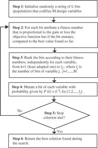
Generalized extremal optimization is an optimization algorithm 3 inspired by a simplified evolutionary model, developed to be easily applicable to a broad class of nonlinear constrained optimization problems, with the presence of any combination of continuous, discrete and integer values for the design variables, while having only one free parameter (γ, see Figure 1) to be adjusted. Its efficacy to tackle complex design spaces has been demonstrated with test functions and real design problems.

Figure 1. The canonical variant of GEO.

3.2. SA algorithm

Based on statistical mechanics reasoning applied to a solidification problem, Metropolis et al. 11 introduced a simple algorithm that can be used to accomplish an efficient simulation of a system of atoms in equilibrium at a given temperature (T). In each step of the algorithm a small random displacement of an atom is performed and the variation of the energy ΔE is calculated. If ΔE < 0 the displacement is accepted, and the configuration with the displaced atom is used as the starting point for the next step. In the case of ΔE > 0, the new configuration can be accepted according to Boltzmann probability (6) where k_B is the Boltzmann's constant.

A uniformly distributed random number r in the interval [0,1] is then calculated and compared with P(ΔE). Metropolis criterion establishes that the new configuration is accepted if r < P(ΔE), otherwise it is rejected and the previous configuration is used again as a starting point. Using the objective function , defined in Equation (3) in place of energy, and defining configurations by a set of variables {Z_i}, i = 1, 2, …, M, see Equation (2) where M = 4 is the total number of unknowns, the Metropolis procedure generates a collection of configurations of a given optimization problem at some temperature T 12. This temperature is simply a control parameter. The simulated annealing process consists of first ‘melting’ the system being optimized at a high-effective ‘temperature’, then lowering the ‘temperature’ until the system ‘freezes’ and no further change occurs.

3.3. GEO + SA algorithm

The GEO + SA hybrid version developed incorporates in GEO the cooling schedule characteristic of the SA 12. In the SA, the stochasticity of the search is determined by the temperature, T, which is constant by stages, and where the definition of the number of stages, the number of function evaluations, and the value of T on each stage defines the cooling schedule. For GEO, the parameter γ defines the stochasticity of the search. Then, the idea is to create for γ a schedule similar to that of SA, generating, in this way, a hybrid algorithm. In the scope of the SA analogy, the temperature defines the amount of energy available in the system and, by consequence, defines the probability of changing from one state to another. In the SA, the higher the temperature, the greater the stochasticity.

In the canonical SA 12, the following equation defines the temperature of a stage: (7) where n is the stage number and q is the temperature reduction rate, or cooling rate, which is a constant such that q = T₁/T₀ = T₂/T₁ = ··· = T_n/T_n−1 and 0 < q < 1.

As q<1, Equation (5) indicates that the parameter T of SA decays exponentially with the stage number, n. As the smaller the temperature, the smaller the search stochasticity, then, the temperature cooling schedule of SA results in a decreasing search stochasticity.

For GEO, the lower the parameter γ, the greater the search stochasticity. Then, in order to achieve the same effects of the SA cooling schedule, the schedule for γ must provide increasing values, instead of decreasing ones. The following equation was formulated having this criterion in mind 4: (8) where γ_MAX is the maximum limit established for γ and n_MAX is the maximum limit for the number of stages, n. Figure 2 shows examples of resulting schedules for n_MAX = 10 and for several values of q.

Figure 2. Scheduling examples for γ.

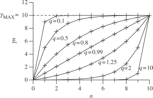
Regarding Equation (6), it is more flexible than the SA schedules, allowing q > 1. As can be seen from Figure 2, schedules with q > 1 have high stochasticity during many stages and low stochasticity during a few stages. When q < 1, the situation is similar to that of SA schedules, where one has high stochasticity during a few stages and low stochasticity during many stages.

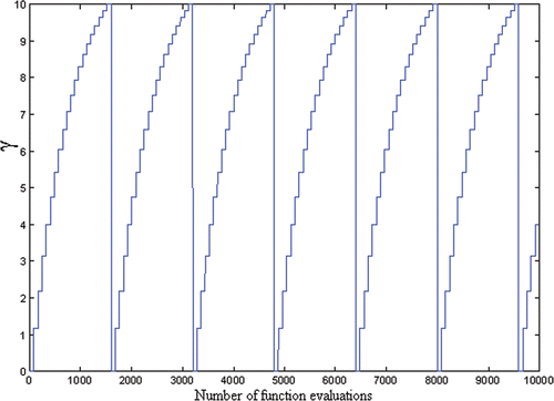
It was decided, in case of GEO + SA, to use exactly L objective function evaluations on each stage. Since GEO requires L objective function evaluations per iteration, a new stage occurs at each algorithm iteration, meaning a new value of γ at each iteration. If the number of algorithm iterations is greater than n_MAX, n is set to zero again and the schedule is restarted, such that several cycles can occur during a search, as exemplified in Figure 3, where six complete cycles occur for n_MAX = 19, q = 0.9 and L = 80. In Figure 3, please note that the vertical lines are not γ actual values. They have been used only for better visualization purposes.

Figure 3. Cyclic scheduling example.

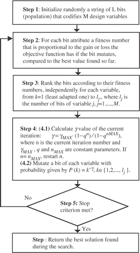
The functionalities just described were incorporated to GEO. Figure 4 brings the resulting GEO + SA hybrid algorithm. It does not have γ as an algorithm parameter. On the other hand, two other parameters appear. They are the number of algorithm iterations per cycle, n_MAX and q, which defines the shape of the schedule. Rigorously speaking, γ_MAX also should be considered as a parameter. However, as γ → γ_MAX must correspond to T → 0, that is, a condition of very low stochasticity, then, it is enough to set for γ_MAX a value that ensures such condition. In this article, the value γ_MAX = 10 was used.

Figure 4. GEO + SA algorithm.

4. Results and discussion

In order to compare GEO + SA performance with the algorithms used in 2, it was applied to the solution of the same inverse radiative transfer problem (described in the Section 2 of this article), and using the same three cases of the former study, as shown in Table 1. GEO + SA used 10 bits to encode each of the unknowns.

Table 1. Exact values of the radiative properties.

Radiative property	Case 1	Case 2	Case 3
Optical thickness, τ0	1.0	2.0	0.5
Single scattering albedo, ω	0.5	0.8	0.3
Diffuse reflectivity, ρ1	0.2	0.1	0.1
Diffuse reflectivity, ρ2	0.2	0.8	0.8

In the same way as in 2, sets of synthetic experimental data were generated with (9) where I_calci represents the calculated values of the radiation intensity using the exact values of the radiative properties, , as given in Table 1, r_i is a pseudo-random number in the range [−1, 1], and σ simulates the standard deviation of the measurement errors. The values of σ = 0.005, 0.002 and 0.0025 lead to the same amount of measurement errors, which are in the order of, or smaller than, 5% in the exit radiation intensities for cases 1, 2, and 3, respectively.

The values of the two parameters of GEO + SA, n_MAX and q, were tuned using all nine combinations from the sets n_MAX ∈ {5, 15, 25} and q ∈ {0.5, 1.01, 2}. For each case, the pairs (n_MAX and q) with the best average results over 10 runs were retrieved and used to be presented in the figures. The runs of GEO + SA were performed on a PC with the processor AMD Athlon 64 (2.2 GHz with 512 MB of RAM). Each run took an average of approximately 45 min.

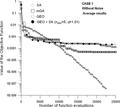
Figure 5 presents the evolution of the average of the best values of the objective function, in 10 runs, and for each method (GEO + SA, GEO, SA and μGA), for Case 1 listed in Table 1, using experimental data without noise, i.e., σ = 0 in Equation (7). In Figure 6 the same test case is considered, but now with noisy data, σ = 0.005.

Figure 5. Average of the best values of the objective function, as a function of the number of function evaluations for Case 1, without noise.

Table 2 presents the worst, average and best estimates obtained for the unknown radiative properties (design variables) in Case 1. Here the worst estimates obtained for each method correspond to the run, among the 10 runs performed for each method, for which the objective function is the highest at the end of the run, and the best estimates correspond to the run for which the value of the function is the lowest.

Figure 6. Average of the best values of the objective function, as a function of the number of function evaluations for Case 1, with noise.

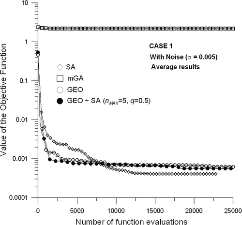
Table 2. Worst, average and best estimates for Case 1.

Exact value			fx^a
SA	Without noise	Worst	6.07 × 10^−8
		Average^b	1.80 × 10^−8
		Best	1.84 × 10^−9
	With noise	Worst	4.03 × 10^−4
		Average^b	4.03 × 10^−4
		Best	4.03 × 10^−4
µGA	Without noise	Worst	2.50 × 10^−4
		Average	4.93 × 10^−5
		Best	2.79 × 10^−6
	With noise	Worst	2.2755
		Average	1.8205
		Best	5.58 × 10^−4
GEO	Without noise	Worst	2.63 × 10^−3
		Average	1.31 × 10^−4
		Best	9.00 × 10^−6
	With noise	Worst	9.46 × 10^−4
		Average	6.16 × 10^−4
		Best	4.37 × 10^−4
GEO + SA	Without noise	Worst	3.05 × 10^−4
		Average	2.15 × 10^−4
		Best	1.39 × 10^−4
	With noise	Worst	6.94 × 10^−4
		Average	5.58 × 10^−4
		Best	4.45 × 10^−4
Notes: ^afx is the value of the objective function at the end of the run. ^bThe SA stopping criterion was reached for all runs in <25,000 evaluations.

Figures 7 and 8, and Table 3 present the results for the Case 2, as defined in Table 1 and using σ = 0 (data without noise) and σ = 0.002 (data with noise).

Figure 7. Average of the best values of the objective function, as a function of the number of function evaluations for Case 2, without noise.

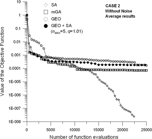
Table 3. Worst, average and best estimates for Case 2.

Exact value			fx^a
SA	Without noise	Worst	1.72 × 10^−8
		Average^b	8.64 × 10^−9
		Best	0.92 × 10^−9
	With noise	Worst	7.76 × 10^−5
		Average^b	7.75 × 10^−5
		Best	7.75 × 10^−5
µGA	Without noise	Worst	1.45 × 10^−4
		Average	7.11 × 10^−5
		Best	7.63 × 10^−6
	With noise	Worst	4.01 × 10^−4
		Average	3.10 × 10^−4
		Best	2.50 × 10^−4
GEO	Without noise	Worst	4.28 × 10^−4
		Average	1.72 × 10^−4
		Best	1.80 × 10^−5
	With noise	Worst	5.21 × 10^−4
		Average	2.62 × 10^−4
		Best	9.90 × 10^−5
GEO + SA	Without noise	Worst	4.94 × 10^−4
		Average	1.86 × 10^−4
		Best	2.37 × 10^−5
	With noise	Worst	3.09 × 10^−4
		Average	1.80 × 10^−4
		Best	8.87 × 10^−5
Notes: ^afx is the value of the objective function at the end of the run. ^bThe SA stopping criterion was reached for all runs in <25,000 evaluations.

For Case 1, it can be seen from the results presented in Figures 5 and 6 that GEO + SA did not performed significantly differently from GEO alone, having objective function evolution curves only marginally different. Without noise, GEO was slightly better than GEO + SA at the end of the search, whereas, with noise, the opposite occurred. For both tests, however, it is possible to notice that GEO + SA is better than GEO early in the search. This advantage early in the search also happens when GEO + SA is compared with the SA. In the end of the search, however, the SA takes the lead with a great margin in the case without noise and a slight one for the case with noise.

Figure 8. Average of the best values of the objective function, as a function of the number of function evaluations for Case 2, with noise.

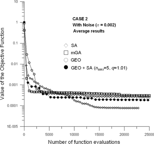
For Case 2, Figures 7 and 8 show that GEO + SA performed slightly better than GEO alone, during greater part of the search. Without noise, GEO and GEO + SA both converged to almost the same value of the objective function in the very end of the search. With noise, GEO + SA kept its advantage over GEO alone during the entire search, having the second best performance among all algorithms. When GEO + SA is compared with the SA, a similar behaviour to the one observed for Case 1 is noticed. That is, GEO + SA is better early in the search for either problems with and without noise, while SA yields a better performance in the long run. Figures 9 and 10, and Table 4 present the results for Case 3, as defined in Table 1 and using σ = 0 (data without noise) and σ = 0.0025 (data with noise).

Figure 9. Average of the best values of the objective function, as a function of the number of function evaluations for Case 3, without noise.

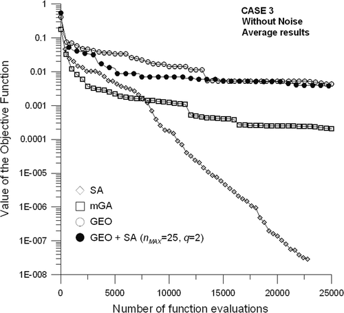
Table 4. Worst, average and best estimates for Case 3.

Exact value			fx^a
SA	Without noise	Worst	3.08 × 10^−8
		Average^b	1.57 × 10^−8
		Best	8.49 × 10^−10
	With noise	Worst	1.08 × 10^−4
		Average^b	1.08 × 10^−4
		Best	1.08 × 10^−4
µGA	Without noise	Worst	5.82 × 10^−4
		Average	2.08 × 10^−4
		Best	2.52 × 10^−5
	With noise	Worst	4.8 × 10^−3
		Average	8.01 × 10^−3
		Best	1.6 × 10^−3
GEO	Without noise	Worst	1.91 × 10^−2
		Average	4.32 × 10^−3
		Best	2.08 × 10^−4
	With noise	Worst	3.31 × 10^−2
		Average	6.82 × 10^−3
		Best	8.17 × 10^−4
GEO + SA	Without noise	Worst	7.86 × 10^−3
		Average	3.86 × 10^−3
		Best	4.54 × 10^−4
	With noise	Worst	3.72 × 10^−3
		Average	2.05 × 10^−3
		Best	1.05 × 10^−3
Notes: ^afx is the value of the objective function at the end of the run. ^bThe SA stopping criterion was reached for all runs in less than 25,000 evaluations.

For Case 3, it can be seen from the results presented in Figures 9 and 10 that GEO + SA performed slightly better than GEO alone in the case without noise. In the case with noise, Figure 10 shows that the GEO + SA curve detached from the GEO alone curve a little before 5000 objective function evaluations and performed considerably better than GEO until the end of the search. When GEO + SA is compared with the SA for Case 3, the last is better with and without noise and during the entire search.

Figure 10. Average of the best values of the objective function, as a function of the number of function evaluations for Case 3, with noise.

5. Conclusions

In the present work, a hybrid version of GEO and SA algorithms was described and its performance on tackling an inverse radiative problem compared to the GEO and SA standalone versions. Called GEO + SA, it achieved mostly a similar or slightly better performance that GEO alone, with the exception of Case 3 with noise, where the hybrid had a clearly better performance than GEO. Compared to the SA stand alone algorithm, the results showed that the latter yields better results, with GEO + SA being superior in some cases, but only early in the search. Ongoing studies are being done in order to verify if, for instance, real instead of binary encoding for the design variables would yield better performance results for GEO + SA.

Acknowledgements

The authors acknowledge CNPq, FAPESP and FAPERJ.

References

- Neto, AJSilva, Explicit and implicit formulations for inverse radiative transfer problems. Presented at 5th World Congress on Computational Mechanics, Mini-Symposium MS 125-Computational Treatment of Inverse Problems in Mechanics. Vienna, Austria, 2002.
- de Sousa, FL, Ramos, FM, Soeiro, FJCP, and Silva Neto, AJ, 2007. Application of the Generalized Extremal Optimization algorithm to an inverse radiative transfer problem, Inverse Probl. Sci. Eng. 15 (–) (2007), pp. 699–714.
- de Sousa, FL, Ramos, FM, Paglione, P, and Girardi, RM, 2003. A new stochastic algorithm for design optimization, AIAA J. 41 (2003), pp. 1808–1818.
- Galski, RL, 2006. Development of improved, hybrid, parallel, and multiobjective versions of the generalized extremal optimization method and its application to the design of spatial systems. D.Sc. Thesis. Instituto Nacional de Pequisas Espaciais, Brazil; 2006, p. 279, INPE-14795-TDI/1238 (In Portuguese).
- Glover, F, Laguna, M, and Martí, R, 2003. Ghosh, A, and Tsutsui, S, eds. Advances in Evolutionary Computation: Theory and Applications. New York: Springer-Verlag; 2003. pp. 519–537.
- Corne, D, Dorigo, M, and Glover, F, 1999. New Methods in Optimization. New York: McGraw Hill; 1999.
- Colorni, A, Dorigo, M, Maffioli, F, Maniezzo, V, Righini, G, and Trubian, M, 1998. Heuristics from nature for hard combinatorial optimization problems, AIAA J 36 (1998), pp. 1105–1112.
- Glover, F, 1977. Heuristics for integer programming using surrogate constraints, Decision Sci. 8 (1977), pp. 156–166.
- Özisik, MN, 1973. Radiative Transfer and Interactions with Conduction and Convection. New York: John Wiley; 1973.
- Chandrasekhar, S, 1960. Radiative Transfer. New York: Dover Publications Inc.; 1960.
- Metropolis, N, Rosenbluth, AW, Rosenbluth, MN, Teller, AH, and Teller, E, 1953. Equation of state calculations by fast computing machines, J. Chem. Phys. 21 (1953), pp. 1087–1092.
- Kirkpatrick, S, Gellat, CD, and Vecchi, MP, 1983. Optimizing by simulated annealing, Science 220 (1983), pp. 671–680.