A response surface method-based hybrid optimizer

Abstract

In this article, we describe a hybrid optimizer based on a highly accurate response surface method, which uses several radial basis functions and polynomials as interpolants. The response surface is capable to interpolate linear as well as highly non-linear functions in multi-dimensional spaces having up to 500 dimensions. The accuracy, robustness, efficiency, transparency and conceptual simplicity are discussed. Based on the extensive testing performed on 296 test functions, the radial basis functions (RBFs) approach seems computationally easy to implement and results are superior, requiring small computing time. The performance of the RBF approximation is compared with wavelets neural networks for several selected test cases and the optimizer is compared with other hybrid optimizers, as well as with the IOSO commercial code.

Keywords:

• hybrid optimization
• multidimensional interpolations
• response surface
• radial basis function polynomials

1. Introduction

The use of RBFs followed by collocation, a technique first proposed by Kansa 1, after the work of Hardy 2 on multivariate approximation, is now becoming an established approach. Various applications to problems in mechanics have been made in recent years – see, for example, Leitão 3,4.

Kansa's method (or asymmetric collocation) starts by building an approximation to the field of interest (normally displacement components) from the superposition of RBFs (globally or compactly supported) conveniently placed at points in the domain and/or at the boundary.

The unknowns (which are the coefficients of each RBF) are obtained from the approximate enforcement of the boundary conditions as well as the governing equations by means of collocation. Usually, this approximation only considers regular RBFs, such as the globally supported multiquadrics or the compactly supported Wendland functions 5.

RBF may be classified into two main groups:

1.	The globally supported ones, namely the multiquadrics (MQ, , where cj is a shape parameter), the inverse multiquadrics, thin plate splines, Gaussians, etc;
2.	The compactly supported ones such as the Wendland 5 family (for example, (1 − r) + n + p(r) where p(r) is a polynomial and (1 − r) + n is 0 for r greater than the support).

There are several other methods for automatically constructing multi-dimensional response surfaces. Notably, a classical book by Lancaster and Salkauskas 6 offers a variety of methods for fitting hypersurfaces of a relatively small dimensionality. Kauffman et al. 7 obtained reasonably accurate fits of data by using second-order polynomials. Ivakhnenko and his team in Ukraine 8 have published an exceptionally robust method for fitting non-smooth data points in multi-dimensional spaces. Their method is based on a self-assembly approach where the analytical description of a hypersurface is a multi-level graph of the type ‘polynomial-of-a-polynomial-of-a-polynomial-of-a- …’ and the basis functions are very simple polynomials. This approach has been used in indirect optimization based upon self-organization (IOSO) 9 commercial optimization software that has been known for its extraordinary speed and robustness.

2. The RBF model

Let us suppose that we have a function of L variables x_i, i = 1, …, L. The RBF model used in this work has the following form (1) where x = {x₁, …, x_i, …, x_L) and f(x) is known for a series of points x. Here, p_k(x_i) is one of the M terms of a given basis of polynomials 10. This approximation is solved for the α_j and β_i,k unknowns from the system of N linear equations, subject to (2) (3)

In this work, the polynomial part of Equation (1) was taken as (4) and the radial basis functions are selected among the following (5) (6) (7) (8) with the shape parameter c_j kept constant as 1/N. The shape parameter is used to control the smoothness of the RBF.

From Equation (1), one can notice that a polynomial of order M is added to the radial basis function. M was limited to an upper value of 6. After inspecting Equations (1–4), one can easily check that the final linear system has [(N + M * L) + 1] equations. Some tests were made using the cross-product polynomials (x_i x_j x_k …), but the improvements on the results were irrelevant. Also, other types of RBFs were used, but no improvement on the interpolation was observed.

The choice of which polynomial order and which RBF are the best for fitting a specific function, was made based on a cross-validation procedure. Let us supose that we have P_TR training points, which are the locations on the multidimensional space where the values of the function are known. Such a set of training points is equally subdivided into two subsets of points, named P_TR1 and P_TR2. Equations (1–3) are solved for a polynomial of order zero and for the RBF expression given by Equations (5–8) using the subset P_TR1. Then, the value of the interpolated function is checked against the known value of the function for the subset P_TR2 and the error is recorded as (9)

Then, the same procedure is made, using the subset P_TR2 to solve Equations (1–3) and the subset P_TR1 to calculate the error as (10)

Finally, the total error for the polynomial of order zero and the RBF expression given by Equations (5–8) is obtained as (11)

This procedure is repeated for all polynomial orders, up to M = 6 and for each one of the RBF expressions given by Equations (5–8). The best combination is the one that returns the lowest value of the RMS error. Although this cross-validation procedure is quite simple, it worked very well for all test cases analysed in this article.

3. Performance measurements

In accordance with having multiple metamodelling criteria, the performance of each metamodelling technique is measured based on the following aspects 11.

•	Accuracy – the capability of predicting the system response over the design space of interest.
•	Robustness – the capability of achieving good accuracy for different problem types and sample sizes.
•	Efficiency – the computational effort required for constructing the metamodel and for predicting the response for a set of new points by metamodels.
•	Transparency – the capability of illustrating explicit relationships between input variables and responses.
•	Conceptual simplicity – ease of implementation. Simple methods should require minimum user input and be easily adapted to each problem.

For accuracy, the goodness of fit obtained from ‘training’ data is not sufficient to assess the accuracy of newly predicted points. For this reason, additional confirmation samples are used to verify the accuracy of the metamodels. To provide a more complete picture of metamodel accuracy, three different metrics are used: R Square (R²), relative average absolute error (RAAE), and relative maximum absolute error (RMAE) 11.

(a) R Square

(12) where is the corresponding predicted value for the observed value y_i; is the mean of the observed values. While MSE (mean square error) represents the departure of the metamodel from the real simulation model, the variance captures how irregular the problem is. The larger the value of R², the more accurate the metamodel.

(b) Relative average absolute error

(13) where STD stands for standard deviation. The smaller the value of RAAE, the more accurate the metamodel.

(c) Relative maximum absolute error

(14)

Large RMAE indicates large error in one region of the design space even though the overall accuracy indicated by R² and RAAE can be very good. Therefore, a small RMAE is preferred. However, since this metric cannot show the overall performance in the design space, it is not as important as R² and RAAE.

Although the R², RAAE and RMAE are useful to ascertain the accuracy of the interpolation, they can fail in some cases. For the R² metric, for example, if one of the testing points has a huge deviation of the exact value, such discrepancy might affect the entire sum appearing in Equation (12) even if all the other testing points are accurately interpolated. Similary, the R² result can be very bad. For this reason, we also calculate the percentage deviation of the exact value of each testing point. Such deviations are collected according to six ranges of errors: 0–10%; 10–20%; 20–50%; 50–100%; 100–200%; >200%. Thus, an interpolation that has all testing points within the interval of 0–10% of relative error might be considered good in comparison to another one where the points are all spread along the intervals from 10% to 200%.

4. Test functions

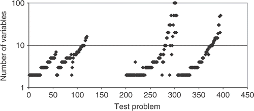
In order to test the accuracy of the RBF model proposed, 296 test cases were used, representing linear and non-linear problems with up to 100 variables. Such problems were selected from a collection of 395 problems (actually 296 test cases), proposed by Hock and Schittkowski 12 and Schittkowski 13. Figure 1 shows the number of variables of each one of the problems. Note that there are 395 problems, but some of them were not used.

Figure 1. Number of variables for each problem considered.

Three methodologies were used to solve the linear algebraic system resulting from Equations (1–3): LU decomposition, SVD and the generalized minimum residual (GMRES) iterative solver. When the number of equations was small (<40), the LU solver was used. However, when the number of variables increased over 40, the resulting matrix becomes too ill-conditioned and the SVD solver had to be used. For more than 80 variables the SVD solver became too slow. Thus, the GMRES iterative method with the Jacobi pre-conditioner was used for all test cases.

In order to verify the accuracy of the interpolation over a different number of training points, three sets were defined. Also, the number of testing points varied, according to the number of training points. Table 1 presents these three sets, based on the number of dimensions (variables) L of the problem.

Table 1. Number of training and testing points.

	Number of training points	Number of testing points
Scarce set	3 L	300 L
Small set	10 L	1000 L
Medium set	50 L	5000 L

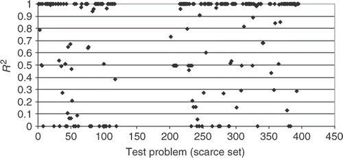
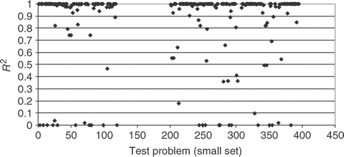
Figure 2 shows the R² metric for all test cases, using the scarce set of training points. It can be noticed that the results are all spread from 0 (completely inadequate interpolation) to 1 (very accurate interpolation). However, even for this very small number of training points, most cases have an excellent interpolation, with R² = 1.

Figure 2. R² metric for the scarce set of training points.

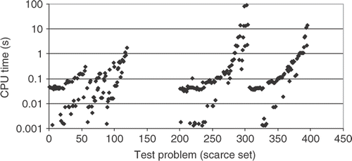
Figure 3 shows the CPU time required to interpolate each test function, using the scarce set of training points. For most of the cases the CPU time was less than 1 s, using an AMD Opteron 1.6 GHz processor and 1 GB Registered ECC DDR PC-2700 RAM. In fact, the highest dimensional test cases, which had 100 variables, required only 100 s to be interpolated.

Figure 3. CPU time for the scarce set of training points.

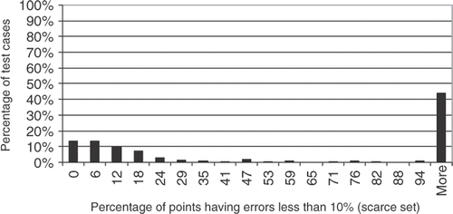
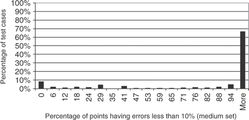
Although the R² might indicate some performance behaviour of the interpolation function, we decided to use a different measure of the accuracy. Figure 4 shows the percentage of testing points having errors less than 10%, against the percentage of all 296 test cases, for the scarce set of testing points. Thus, from Figure 4, it can be noticed that for more than 40% of all test functions, the relative errors were less than 10%. This is a very good result, considering the extremely small number of training points used in the scarce set.

Figure 4. Testing points with less than 10% error, for the scarce set of training points.

Figure 5 shows the R² metric for the small set of training points. Comparing with Figure 2, it can be seen that the points move toward the value of R² = 1.0, showing that the accuracy of the interpolation gets better when the number of training points increase.

Figure 5. R² metric for the small set of training points.

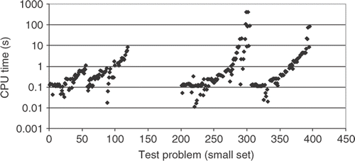
Figure 6 shows the CPU time required for all test cases, when the small number of training points is used. Although the test case with 100 variables requires almost 1000 s, in almost all test cases the CPU time is low.

Figure 6. CPU time for the small set of training points.

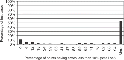
Figure 7 shows the percentage of points having errors lower than 10%. Comparing with Figure 4, one can see that increasing the number of training points from 3L (scarce set) to 10 L (small set), the number of testing points having less than 10% of relative error for all 296 test cases increase from ∼45% to ∼55%, showing a very good interpolation, even for a not so large number of training points.

Figure 7. Testing points with less than 10% error, for the small set of training points.

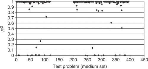
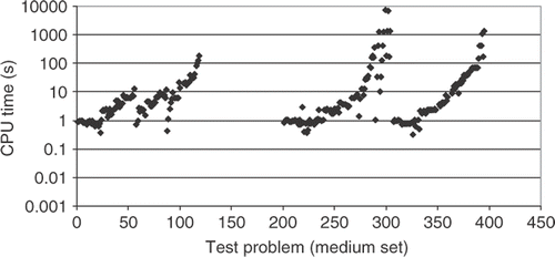
Finally, Figures 8–10 show the results when a medium set of training points are used. From Figure 8, one can notice that the majority of the test cases have the R² metric close to 1.0, indicating a very good interpolation, for a not so large CPU time, as it can be verified from Figure 9. From Figure 10, the number of testing points having errors less than 10% for all 296 test cases increases to ∼75% when a medium (50 L) number of training points is used. This indicates that such interpolation can be used as a meta model in a optimization task, where the objective function takes too long to be calculated. Thus, instead of optimizing the original function, an interpolation can be used, reducing significantly the computational time.

Figure 8. R² metric for the medium set of training points.

Figure 9. CPU time for the medium set of training points.

Figure 10. Testing points with less than 10% error, for the medium set of training points.

5. Comparison with another method of interpolation

In order to compare the current RBF interpolation procedure, which is proposed here, we compared its performance against another method. The second method used for fitting high-dimensional functions was the wavelets-based neural network (WNN) model presented by Sahoo and Dulikravich 14 with five neural subnets. Training the WNN for response surface generation was done using a random sequence dataset of Sobol and Levitan 15. Typically, the mother wavelet used in the WNN is Mexican Hat wavelet given by: (15)

Gaussian wavelets were also used along with this mother wavelet to construct the WNN. For each node of the WNN, genetic algorithm was used to search the best Mexican Hat wavelet and the best Gaussian wavelet. The one having a lower norm of residue after performing multiple linear regressions was selected and used in the WNN architecture.

In order to test the accuracy of the RBF model proposed, 13 test cases were used, representing linear and non-linear problems with up to 16 variables. These test cases, defined as problems 1–13 were selected by Jin et al. 11 in a comparative study among different kinds of meta-models. Such problems were selected from a collection of 395 problems (actually 296 test cases), proposed by Hock and Schittkowski 12 and Schittkowski 13. The first 12 problems do not have random errors added to the original function, while the problem no. 13 has a noise added with the following form: (16)

where σ is the standard deviation and r is a random number with Gaussian distribution and zero mean.

The RBF model presented here was based on the multiquadrics – Equation (5) – and only the polynomial order was varied. Such interpolant was compared against the WNN method for the 13 selected test cases. Table 2 gives the number of training points, testing points, minimum and maximum value of each test function, as well as the standard deviation and average value of each test function.

Table 2. Parameters for the 13 test functions.

		Number of training and testing points
		Training
PB #	# Vars	Scarce	Small	Large	Testing	Non Linearity	Minimum value of f	Maximum value of f	Standard deviation of f	Average value of f
PB1	10	30	100	198	1000	High	−21.01	29.25	8.92	8.60
PB2	10	30	100	198		Low	−1717.43	−539.36	187.40	−1146.82
PB3	10	30	100	198		High	−1327241.16	−1.14	224561.73	−213124.84
PB4	10	30	100	198		Low	258.78	4779.01	1002.27	2185.25
PB5	16	48	160	459		Low	7136.99	195608.81	27294.72	69060.73
PB6	2	N/A	9	100		High	98.94	187.53	17.75	127.73
PB7	2		9	100		High	−0.26	0.26	0.15	0.00
PB8	2		9	100		Low	−1.51	8.91	2.08	1.66
PB9	3		27	125		High	2.15	146369.38	21527.31	10842.11
PB10	3		27	125		High	3.42	32.84	7.70	29.13
PB11	3		27	125		Low	−40829.97	−40749.42	21.60	−40790.41
PB12	2		9	100		Low	−12.72	13.75	5.74	0.52
PB13	2		9	100		Low	−54.77	77.80	30.94	12.60

In order to check the accuracy of the metamodel when different samples were employed, three different sets of training points were used, as suggested by Jin et al. 11.

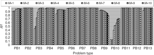
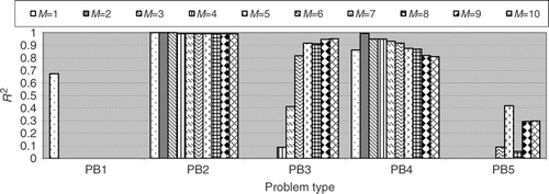
Initially, the accuracy of the RBF expansion was tested for a large set of training points as defined in Table 2. Figure 11 shows the results for different orders of the polynomial, part of the RBF expansion are presented in Equations (1–3). From Figure 11 one can see that by increasing the order of the polynomial the results become much better except for the problem no. 9, where the R² metric decreases when M increases. In fact, for all problems, except no. 10, the RBF expansion achieves the R² metric over 0.9, showing a very good global accuracy. Therefore, for a large set of training points a high polynomial order should be used in order to achieve high accuracy.

Figure 11. Influence of the polynomial order on the R² metric for a large set of training points.

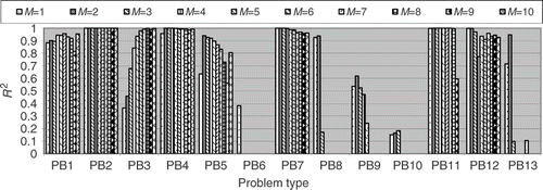
Next, the same comparison was made for a small number of training points, as defined in Table 2. Figure 12 shows the results of the R² metric for this comparison. It can be observed that problem no. 1 is almost insensitive to the order of the polynomial, except for M = 9.

Figure 12. Influence of the polynomial order on the R² metric for a small set of training points.

Problem no. 11 is also insensitive except for M greater than 8, where the performance drops rapidly. Problems no. 2 and 4 are insensitive to the value of M, while problem no. 7 shows a small decrease of the R² value for high-order polynomials. Problem no. 3 shows an increase in the R² values when M increases, just as in the case with a large set of training points. However, problems no. 5, 6, 9, 10 and 13 show a drop in the R² value when the polynomial order is increased so that some metrics were way below zero. From Figure 12, in order to keep the method robust we conclude that, if the number of training points is small, the order of the polynomial should be kept small.

Figure 13 shows the comparison of the R² metrics for several polynomial orders for a scarce set of training points. Only problems no. 1–5 were tested for a scarce set of training points, as suggested by Jin et al. 11. Problems no. 2 and 3 have the same behaviour as for a small set of training points. However, problem no. 1 rapidly drops its value of R² for a high polynomial order. Again, the minimum value of the scale was limited to zero, because some of the R² values were way below zero. The performance of problem no. 5 oscillates when M is varied. Again, we concluded that for a scarce number of training points, a lower polynomial order should be used in order to keep the method more robust.

Figure 13. Influence of the polynomial order on the R² metric for a scarce set of training points.

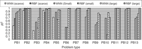
Next, the results obtained with a RBF polynomial of order 10 using a large number of training points and the results obtained with a polynomial of order 1 for small and scarce sets of training points were compared with the results obtained by using WNN method 14. Again, only problems no. 1–5 were tested for a scarce set of training points, as suggested by Jin et al. 11.

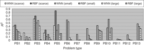
The results for the R² metric are presented in Figure 14, where one can see that the RBF formulation performed better than the WNN for a scarce number of training points for problems no. 1 and 2. For problem no. 4 the value of R² is a little small for the RBF when compared to WNN. For problems no. 3 and 5 the RBF performed quite poorly, while the WNN was able to obtain some results. For a small set of training points the RBF was better than the WNN for problems no. 1, 7, 8, 9, 12 and 13, while the WNN performed better for problems no. 3, 5, and 10. The performance was practically the same for problems no. 2, 4, 6 and 11. For a large number of training points the WNN performed better for problems no. 9 and 10, while the RBF had a better performance for problems no. 1, 3 and 13. For problems no. 2, 4, 5, 6, 7, 8, 11 and 12 the accuracy of both methods was almost the same. Figure 15 shows the comparisons of RAAE for all 13 test functions, both for RBF and WNN. Recall that for this metric lower values are better than high values. For a scarce set of training points the RBF performed better for problem no. 2, while the WNN was better for problems no. 2, 3 and 4. For problem no. 1 RAAE values for both of the methods were comparable.

Figure 14. R² metric for WNN and RBF.

Figure 15. RAAE metric for WNN and RBF.

It is interesting to note that the R² value for problems no. 3 and 4 (Figure 14) were bad when the RBFs were used. However, the RAAE metrics for these two problems are better when compared to the WNN. Actually, the RAAE metric for problem no. 3 is ∼15% greater for RBF than for WNN, while the R² metrics for this problem was under zero for RBF. For small set of training points the RBF performed better for problems no. 1, 2, 6, 7, 8, 9, 12 and 13, while the WNN performed better for problems no. 3, 4, 5 and 10. The values of RAAE for both methods were almost equal for problem no. 11. For a large set of training points the RBF performed better than the WNN, except for problems no. 5 and 10. Thus, as it was observed in the R² metric, for large and small sets of training points, the RBF was better than the WNN, while for a scarce number of training points, the WNN performed better.

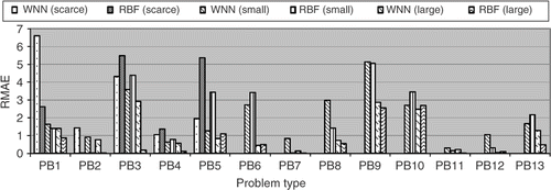
Finally, Figure 16 shows the results for the RMAE for all 13 test functions. A high value of the RMAE means a bad local estimate. For a scarce set of training points the general trend is very close to the previous one, related to the RAAE metric, showing a better performance for RBF in the problem no. 2, while the WNN performed better for problems no. 3–5. However, for problem no. 1, the RBF performed much better than WNN, indicating that the WNN had some inaccurate local estimates. For a small set of training points the RBF performed better for problems no. 2, 7, 8 and 12, while the WNN performed better for problems no. 3, 5, 6, 10 and 13. For problems no. 1, 4, 9 and 11 the values of RMAE were close to each other. For a large set of training points the RBF was better for problems no. 1–4, 7–9, 11 and 13, while the WNN was better for the problems no. 5 and 10. For problems no. 6 and 12 the performance was practically the same for both of them.

Figure 16. RMAE metric for WNN and RBF.

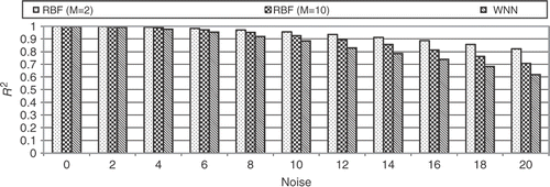
In order to check the robustness of the two models when noise is added, test problem no. 13 was used with several values of σ. For this test 100 training points and 1000 testing points were used. Figure 17 shows how the R² metric decreases when the added noise in the original function increases. It is worth to note that the RBF performed better than the WNN. In fact, even for a high level of noise, the RBF still shows a value of 0.8 for the R² metric when the order of the polynomial is equal to M = 2. It is quite interesting that when no noise is added, the R² metric decreases when the order of the polynomial increases, which is exactly the opposite trend to the one presented in Figure 11 for the function number 13 without noise.

Figure 17. Influence of noise on the R² metric.

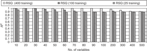
Finally, a test case with progressively large number of variables was proposed. For this test case test function no. 2 was chosen with 25, 100 and 400 training points and 1000 testing points for various problem dimensions. Figure 18 shows the results for the R² metrics when the RBF was used with a polynomial of order M = 10. It is surprising that the RBF is able to maintain a high level of R², even for a problem with 500 variables. It is worth noting that when the number of training points decreases, the value of R² also decreases, but not significantly.

Figure 18. R² results for a large number of variables (RBF with M = 10).

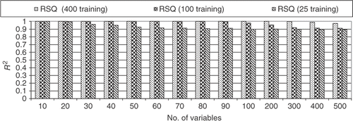
Figure 19 shows the results for the same test case presented in Figure 18, but now for a polynomial of order M = 1. Since it was observed in Figures 11–13, the problem no. 2 is insensitive to the order of the polynomial for scarce, small and large set of training points. It is interesting to note the similar results when a high-order polynomial was used (Figure 18). In fact, the results are even better for 500 variables.

Figure 19. R² results for a large number of variables (RBF with M = 1).

The reason for this is that the linear system resulting from the RBF approximation has [(N + M * L) + 1] equations, where N is the number of training points, L is the number of variables and M is the order of the polynomial. Thus, when a high-order polynomial is used, the matrix becomes too large and might become more ill-conditioned.

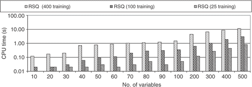
Finally, Figure 20 shows the computational time required to run this test case. It is quite surprising that the computational time was lower than 10 s for all test cases, meaning that the RBF approximation is very fast. The code was written in Fortran 90 and the CPU was an Intel T2300 1.66 GHz (Centrino Duo) with 1 Gb RAM.

Figure 20. CPU time for a large number of variables (RBF with M = 1).

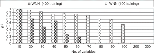
Figure 21 shows the results for test problem no. 2 for a large number of variables, using the WNN. One can see that the accuracy, given by the R² metric, decreases rapidly when using 100 training points. Also, for 400 training points, the R² goes to a negative value for more than 100 variables, while the RBF (see Figures 18 and 19) maintains good accuracy even when there are 500 variables.

Figure 21. R² results with WNN for a large number of variables (WNN with five subnets).

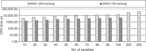
Figure 22 shows the computational time required by the WNN where one can notice the high computational cost. In fact, for 100 variables, the time required was about 4 h, while for 300 variables it was more than 11 h. The code for the WNN was written in Matlab 7.0.4 and the CPU was an Intel T2300 1.66 Ghz (Centrino Duo) with 1 Gb RAM. Some improvement in the performance can be obtained by converting this code to Fortran90 or C++ and this should be investigated. However, the computational cost for the WNN for a problem with 300 variables and 400 training points, even with different languages (Matlab and Fortran90) was ∼6000 times greater for the RBF.

Figure 22. CPU time for a large number of variables (WNN with five subnets).

Finally, the same problem was run again using WNN with only one sub-net and 400 training points, using the Mexican Hat function. The results are presented in Figure 23.

Figure 23. R² results and CPU time for a large number of variables (WNN with one subnet).

One can see that the computational time decreases when compared with the ones presented in Figure 22 by a factor of five, but the R² metrics also decreases. It is interesting to note that, again, after 100 variables, the R² metrics goes to a negative value when the WNN is used. Thus, it is not recommended to reduce the number of neural sub-nets in order to speed-up the training process, because the accuracy goes down. In conclusion, at least for the problem no. 2, the RBF is more robust than the WNN when a very large number of variables is used.

6. The new hybrid optimizer

Based on the previous results of the RBF, we proposed a hybrid optimizer which uses a response surface instead of the real objective function. The RBF used was the one described in Section 2 of this article. This hybrid optimizer was compared against our previously developed ones 16–18 and the IOSO commercial code 9 for some well-known test functions.

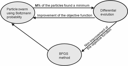
The old hybrid optimizers will be called H1 and H2. A hybrid optimization is a combination of the deterministic and the evolutionary/stochastic methods, in the sense that it utilizes the advantages of each of these methods. The hybrid optimization method usually employs an evolutionary/stochastic method to locate a region where the global extreme point is located and then automatically switches to a deterministic method to get to the exact point faster. The hybrid optimization method H1 16,17 is quite simple conceptually, although its computational implementation is more involved. The global procedure is illustrated in Figure 24. It uses the concepts of four different methods of optimization, namely: the Broyden–Fletcher–Goldfarb–Shanno (BFGS) quasi-Newton method 19, the particle swarm method 20, the differential evolution method 21 and the simulated annealing method 22.

Figure 24. Global procedure for the hybrid optimization method H1.

In order to speed-up the optimization task, in real life problems a multilevel approach is utilized, where the procedure illustrated in Figure 24 is repeated over several levels of grid refinement. Thus, the optimization procedure starts with a very coarse grid and it goes to a finer grid as the iteration continues.

The driven module is the particle swarm method, which performs most of the optimization task. The particle swarm method is a non-gradient-based optimization method created in 1995 by an electrical engineer (Russel Eberhart) and a social psychologist (James Kennedy) 20 as an alternative to the genetic algorithm methods. This particle swarm method is based on the social behaviour of various species and tries to equilibrate the individuality and sociability of the individuals in order to locate the optimum of interest. The original idea of Kennedy and Eberhart came from the observation of birds looking for a nesting place. When the individuality is increased, the search for alternative places for nesting is also increased. However, if the individuality becomes too high the individual might never find the best place. In other words, when the sociability is increased, the individual learns more from their neighbour's experience. However, if the sociability becomes too high, all the individuals might converge to the first place found (possibly a local minimum).

In the particle swarm method, the iterative procedure is given by (17) (18) where

	xi is the i-th individual of the vector of parameters.
	vi = 0, for k = 0.
	r1i and r2i are random numbers with uniform distribution between 0 and 1.
	pi is the best value found for the vector xi.
	pg is the best value found for the entire population.
	0 < α < 1; 1 < β < 2

In Equation (18), the second term on the right-hand side represents the individuality and the third term represents the sociability. The first term on the right-hand side represents the inertia of the particles and, in general, must be decreased as the iterative process proceeds. In this equation, the vector p_i represents the best value ever found for the i-th component of vector of parameters x_i during the iterative process. Thus, the individuality term involves the comparison between the current value of the i-th individual x_i and its best value in the past. The vector p_g is the best value ever found for the entire population of parameters (not only the i-th individual). Thus, the sociability term compares x_i with the best value of the entire population in the past.

The differential evolution method 21 is an evolutionary method based on Darwin's theory of evolution of the species. This non-gradient-based optimization method was also created in 1995 as an alternative to the genetic algorithm methods. Following Darwin's theory, the strongest members of a population will be more capable of surviving under a certain environmental condition. During the mating process, the chromosomes of two individuals of the population are combined in a process called crossover. During this process mutations can occur, which can be good (individual with a better objective function) or bad (individual with a worse objective function). The mutations are used as a way to escape from local minima. However, their excessive usage can lead to a non-convergence of the method.

The method starts with a randomly generated population matrix P in the domain of interest. Thus, successive combinations of chromosomes and mutations are performed, creating new generations until an optimum value is found.

The iterative process is given by (19) where

	xi is the i-th individual of the vector of parameters.
	α, β and γ are three members of population matrix P, randomly chosen.
	F is a weight function, which defines the mutation (0.5 < F < 1).
	k is a counter for the generations.
	δ1 and δ2 are delta Dirac functions that define the mutation.

In this minimization process, if f(x^k+1) < f(x^k), then x^k+1 replaces x^k in the population matrix P. Otherwise, x^k is kept in the population matrix.

The binomial crossover is given as (20) where CR is a factor that defines the crossover (0.5 < CR < 1) and R is a random number with uniform distribution between 0 and 1.

In the hybrid optimizer H1, when a certain percentage of the particles find a minimum, the algorithm switches automatically to the differential evolution method and the particles are forced to breed. If there is an improvement in the objective function, the algorithm returns to the particle swarm method, meaning that some other region is more prone to have a global minimum. If there is no improvement on the objective function, this can indicate that this region already contains the global value expected and the algorithm automatically switches to the BFGS method in order to find its location more precisely. In Figure 4, the algorithm returns to the particle swarm method in order to check if there are no changes in this location and the entire procedure repeats itself. After some maximum number of iterations is performed (e.g., five) the process stops.

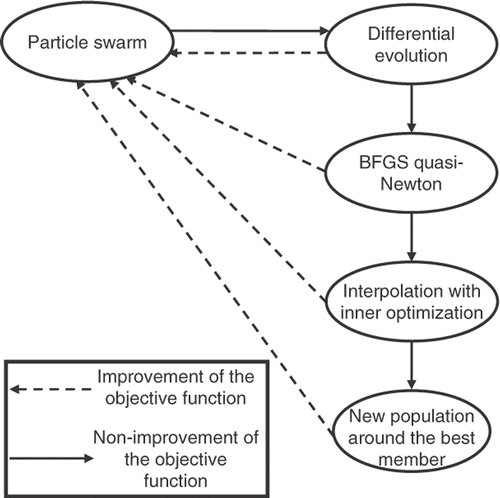
The hybrid optimizer H2 18 is quite similar to the H1, except by the fact that it uses a response surface method at some point of the optimization task. The global procedure is illustrated in Figure 25. It can be seen from Figure 25 that after a certain number of objective functions were calculated, all this information was used to obtain a response surface. Such a response surface is then optimized using the same proposed hybrid code defined in the H1 optimizer so that it fits the calculated values of the objective function as closely as possible. New values of the objective function are then obtained very cheaply by interpolating their values from the response surface.

Figure 25. Global procedure for the hybrid optimization method H2.

In Figure 25, if the BFGS cannot find any better solution, the algorithm uses a radial basis function interpolation scheme to obtain a response surface and then optimizes such response surface using the same hybrid algorithm proposed. When the minimum value of this response surface is found, the algorithm checks to see if it is also a solution of the original problem. Then, if there is no improvement of the objective function, the entire population is eliminated and a new population is generated around the best value obtained so far. The algorithm returns to the particle swarm method in order to check if there are no changes in this location and the entire procedure repeats itself. After a specified maximum number of iterations is performed (e.g., five) the process stops.

The new algorithm, presented at this article, which will be called H3 is an extension of the previous ones. The global procedure is enumerated below:

1.	Generate an initial population, using the real function (not the interpolated one) f(x). Call this population Preal.
2.	Determine the individidual that has the minimum value of the objective function over the entire population Preal and call this individual xbest.
3.	Determine the individual that is more distante from the xbest, over the entire population Preal. Call this individual xfar.
4.	Generate a response surface, with the methodology in Section 2, using the entire population Preal as training points. Call this function g(x).
5.	Optimize the interpolated function g(x) using the hybrid optimizer H1, defined above, and call the optimum variable of the interpolated function as xint. During the generation of the internal population to be used in the H1 optimizer, consider the upper and lower bounds limits as the minimum and maximum values of the population Preal in order to not extrapolate the response surface.
6.	If the real objective function f(xint) is better than all objective function of the population Preal, replace xfar by xint. Else, generate a new individual, using the sobol pseudo-random generator within the upper and lower bounds of the variables, and replace xfar by this new individual.
7.	If the optimimum is achieved, stop the procedure. Else, return to step 2.

From the above sequence, one can notice that the number of times that the real objective function f(x) is called is very small. Also, from step 6, one can see that the space of search is reduced at each iteration. When the response surface g(x) is no longer capable of finding a minimum, a high fidelity evaluation of the real function f(x) is made to generate a new point to be included in the interpolation. Since the CPU time to calculate the interpolated function is very small, the maximum number of iterations of the H1 optimizer can be very large (e.g. 1000 iterations).

The hybrid optimizer H3 was compared against the optimizer H1, H2 and the commercial code IOSO 2.0 for some standard test functions. The first test function was the Levy #9 function 23, which has 625 local minima and 4 variables. Such function is defined as (21) where (22)

The function is defined within the interval −10 ≤ x ≤ 10 and its minimum is f(x) = 0 for x = 1. Figure 26 shows the optimization history of the IOSO, H1–H3 optimizers. Since the H1–H3 optimizers are based on random number generators (because of the particle swarm module), we present the best and worst estimates for these three optimizers.

Figure 26. Optimization history of the Levy #9 function for the (a) IOSO, (b) H1-best, (c) H2-best, (d) H3-best, (e) H1-worst, (f) H2-worst and (g) H3-worst optimizers.

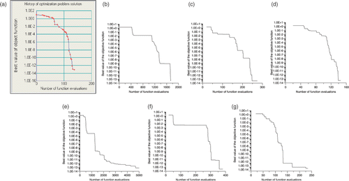
From Figure 26, it can be seen that the performance of the H3 optimizer is very close to the IOSO commercial code. The H1 code is the worst and the H2 optimizer also has a reasonably good performance. It is interesting to note that the H1 code is the only one that does not have a response surface model implemented.

The second function tested was the Griewank function 17, which is defined as (23)

The global minima for this function is located at x = 0 and is f(x) = 0. The function has a very large number of local minima, making the optimization task quite difficult.

Figure 27 shows the optimization history of the IOSO, H1–H3 optimizers. Again, the best and worst results for H1–H3 are presented.

Figure 27. Optimization history of the Griewank function for the (a) IOSO, (b) H1-best, (c) H2-best, (d) H3-best, (e) H1-worst, (f) H2-worst and (g) H3-worst optimizers.

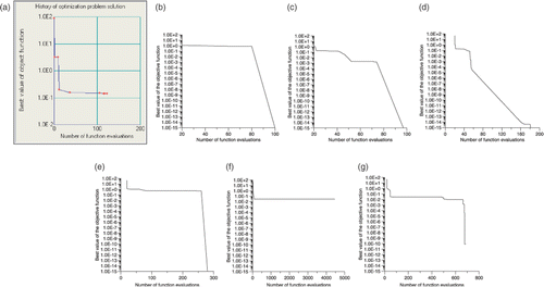
From this Figure 27, it is clear that the H1–H3 optimizers are much better than the IOSO commercial code. The H1 code was the best, while the H2 sometimes stopped at some local minima. The worst result of the H3 optimizer was, however, better than the result obtained by IOSO. It is worth noticing that, with more iterations, the H3 code could reach the minimum of the objective function, even for the worst result.

The next test function implemented was the Rosenbrook function 24, which is defined as (24)

The function is defined within the interval −10 ≤ x ≤ 10 and its minimum is f(x) = 0 for x = 1. Figure 28 shows the optimization history of the IOSO, H1–H3 optimizers.

Figure 28. Optimization history of the Rosenbrook function for the (a) IOSO, (b) H1-best, (c) H2-best, (d) H3-best, (e) H1-worst, (f) H2-worst and (g) H3-worst optimizers.

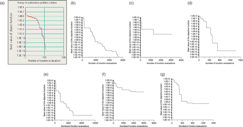
For this function, which is almost flat close to the global minima, the IOSO code was the one with the best performance, followed by the H3 optimizer. The H2 performed very bad and the H1 was able to get close to the minimum, but with a huge number of objective function calculations. When looking at the H3 results, the final value of the objective function differ by some orders of magnitude. However, the optimum solution obtained with this new optimizer was x₁ = 0.9996 and x₂ = 0.9992, while the IOSO obtained x₁ = 1.0000 and x₂ = 1.0000. Thus the relative error among the variables was less than 0.01%, indicating that despite of the discrepancy among the final value of the objective function, the H3 code was able to recover the value of the optimum variables with a negligible relative error.

The last test function analysed was the Mielle–Cantrel function 25, which is defined as (25)

The function is defined within the interval −10 ≤ x ≤ 10 and its minimum is f(x) = 0 for x₁ = 0 and x₂ = x₃ = x₄ = 1. Figure 29 shows the optimization history of the IOSO, H1–H3 optimizers. Again, the best and worst results for H1–H3 are presented.

Figure 29. Optimization history of the Mielle-Cantrel 25 function for the (a) IOSO, (b) H1-best, (c) H2-best, (d) H3-best, (e) H1-worst, (f) H2-worst and (g) H3-worst optimizers.

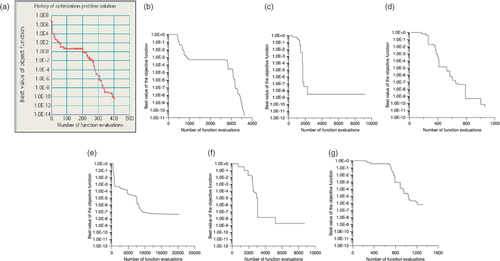
For this function, the IOSO code was the best, followed by the H3. The H2 code performed very badly. Again, the H1 was able to get to the global mininum after a huge numbe of objective function calculations. As occurred with the Rosenbrook function, in spite of the H3 result for the objective function differing from the IOSO code, the final values of the variables were x₁ = 4.0981 × 10⁻⁸, x₂ = 0.9864, x₃=0.9688 and x₄=0.9626 for the H3 optimizer and x₁ = −0.1216 × 10⁻⁵, x₂ = 1.002, x₃ = 0.9957 and x₄ = 0.9962 for the IOSO code.

7. Conclusions

In this work, we presented an interpolation procedure based on radial basis functions. The procedure was shown to work on highly non-linear functions where a large number of variables were involved. The RBF technique seems to be quite powerful regarding its accuracy and reduced CPU time. Even when the number of variables was as large as 500, the RBF approximation was very fast and robust. This is a promising technique for real-time interpolations such as target tracking or image recognition. Some comparisons were made with the WNN showing a general superior behaviour of the RBF. A new hybrid optimizer based on the RBF interpolation was also presented, which is much more efficient than our previous ones. In fact, its performance is very close to one of the best commercial optimizers available.

Acknowledgements

This work was partially funded by CNPq and FAPERJ (Brazilian councils for scientific development). The author is very grateful for the financial support from FIU as well as the hospitally of the Dulikravich family during his stay in Miami from September to November 2006.

References

- Kansa, EJ, 1990. Multiquadrics – a scattered data approximation scheme with applications to computational fluid dynamics – II: solutions to parabolic, hyperbolic and elliptic partial differential equations, Comput. Math. Appl. 19 (1990), pp. 149–161.
- Hardy, RL, 1971. Multiquadric equations of topography and other irregular surfaces, J. Geophys. Res. 176 (1971), pp. 1905–1915.
- Leitão, VMA, 2001. A mesheless method for Kirchhoff plate bending problems, Int. J. Num. Methods Eng. 52 (2001), pp. 1107–1130.
- 2004. RBF-based meshless methods for 2D elastostatic problems, Eng. Anal. Boundary Elements 28 (2004), pp. 1271–1281.
- Wendland, H, 1998. Error estimates for interpolation by compactly supported radial basis functions of minimal degree, J. Approx. Theory 93 (1998), pp. 258–272.
- Lancaster, P, and Salkauskas, K, 1986. Curve and Surface Fitting: An Introduction. Harcourt Brace Jovanovic, London, San Diego, New York: Academic Press; 1986.
- Kaufman, M, Balabanov, V, Burgee, SL, Giunta, AA, Grossman, B, Mason, WH, Watson, LT, and Haftka, RT, 1996. Variable complexity response surface approximations for wing structural weight in HSCT design. Presented at AIAA Paper 96-0089, Proceedings of the 34th Aerospace Sciences Meeting and Exhibit.
- Madala, HR, and Ivakhnenko, AG, 1994. Inductive Learning Algorithms for Complex Systems Modeling. Boca Raton, Florida: CRC Press; 1994.
- IOSO NM, 2003. Version 1.0, User's Guide. Moscow, Russia: IOSO Technology Center; 2003.
- Buhmann, MD, 2003. Radial basis functions on grids and beyond. Lisbon: International Workshop on Meshfree Methods; 2003.
- Jin, R, Chen, W, and Simpson, TW, Comparative studies of metamodeling techniques under multiple modeling criteria. Presented at Proceedings of the 8th AIAA/USAF/NASA/ISSMO Multidisciplinary Analysis & Optimization Symposium, AIAA 2000-4801. Long Beach, CA, 6–8 September, 2000.
- Hock, W, and Schittkowski, K, 1981. Test Examples for Nonlinear Programming Codes, Lecture Notes in Economics and Mathematical Systems. Vol. 187. Berlin, Heidelberg, New York: Springer-Verlag; 1981.
- Schittkowski, K, 1987. More Test Examples for Nonlinear Programming, Lecture Notes in Economics and Mathematical Systems. Vol. 282. Berlin: Springer Verlag; 1987.
- Sahoo, D, and Dulikravich, GS, Evolutionary wavelet neural network for large scale function estimation in optimization. Presented at AIAA Paper AIAA-2006-6955, 11th AIAA/ISSMO Multidisciplinary Analysis and Optimization Conference. Portsmouth, VA, 6–8 September, 2006.
- Sobol, IM, and Levitan, YL, 1976. The Production of Points Uniformly Distributed in a Multidimensional Cube. Moscow, Russia: Preprint IPM Akademia Nauk SSSR; 1976, Number 40.
- Colaço, MJ, Orlande, HRB, and Dulikravich, GS, 2004. Inverse and optimization problems in heat transfer, J. Braz. Soc. Mech. Sci. Eng. XXVIII (1) (2004), pp. 1–23.
- Colaço, MJ, 2005. "Hybrid optimization with automatic switching among optimization algorithms". In: Annicchiarico, W, Periaux, J, Cerrolaza, M, and Winer, G, eds. Handbooks on Theory and Engineering Applications of Computational Methods: Evolutionary Algorithms and its Applications. CIMNE, Barcelona, Spain, UK: WIT Press; 2005. pp. 92–118.
- Colaço, MJ, and Dulikravich, GS, 2007. Solidification of double-diffusive flows using thermo-magneto-hydrodynamics and optimization, Mater. Manufact. Process 22 (2007), pp. 594–606.
- Broyden, CG, 1987. Quasi-Newton methods and their applications to function minimization, Math. Comp. 21 (1987), pp. 368–380.
- Kennedy, J, and Eberhart, RC, 1995. Particle swarm optimization. Presented at Proceedings of the 1995 IEEE International Conference on Neural Networks.
- Storn, R, and Price, KV, 1996. Minimizing the real function of the ICEC’96 contest by differential evolution. Presented at Proceedings of IEEE Conference on Evolutionary Computation.
- Corana, A, Marchesi, M, Martini, C, and Ridella, S, 1987. Minimizing multimodal functions of continuous variables with the ‘Simulated Annealing Algorithm’, ACM Trans. Math. Software 13 (1987), pp. 262–280.
- More, JJ, Garbow, BS, and Hillstrom, KE, 1981. Fortran subroutines for testing unconstrained optimization software, ACM Trans. Math. Software 7 (1) (1981), pp. 17–41.
- Sandgren, E, 1977. The utility of nonlinear programming algorithms, PhD Thesis. Indiana, USA: Purdue University; 1977.
- Miele, A, and Cantrell, JW, 1969. Study on a memory gradient method for the minimization of functions, J. Optim. Theory Appl. 3 (6) (1969), pp. 459–470.