Abstract
In this article, we investigate both analytical and numerical techniques for the identification of the constant perfusion coefficient in the transient bio-heat conduction equation. In this inverse coefficient identification problem, the additional measurement necessary to render a unique solution may be a heat flux, an interior temperature or an average temperature measurement at a single instant. Numerical results obtained using the boundary element method combined with an ordinary non-linear minimization are presented and discussed.
1. Introduction
The study of biomedical heat transfer is not only important in theoretical aspects but also in practical applications Citation1. In particular, the bio-heat conduction equation has been applied for modelling hyperthermia, thrombosis and vascular sclerosis Citation2.
In 1948, Pennes postulated that the effect of the temperature difference between the blood supply and the tissue acts as an energy sink term Citation3. This, in essence, is very similar to the heat transfer fin equation where the sink term represents convective heat loss to the surrounding.
The bio-heat transfer equation proposed by Pennes Citation3, can be written in dimensional form as
(1)
where T* is the temperature of the tissue,
is the temperature of the arterial blood, wb is the blood perfusion rate, Cb is the heat capacity of blood, ρt, ct and kt are the density, specific heat and thermal conductivity of the tissues, respectively, t* is the time, Ω* is the spatial solution domain and S* is a volumetric heat source containing heat generation due to metabolism and heat deposition.
Introducing the dimensionless variables
(2)
where
is a characteristic length of the biological tissue, αt = kt/ρtct is the thermal diffusivity of the tissue and S0 is an average volumetric heat source, then the governing Equation (1) can be expressed in dimensionless form as Citation4,Citation5,
(3)
where
(4)
Equation (3) has to be solved subject to appropriate initial and boundary conditions and if Ω, Pf and S are specified, then this gives rise to a well-posed problem, see Citation6 for a review of numerical solutions. However, in practice, often the coefficient Pf, the heat source S or parts of the boundary ∂Ω come from measurements that may be inaccurate or inaccessible if a hostile environment is present. Therefore, in this article we investigate the inverse problem, which requires finding the coefficient Pf > 0, i.e. from Equation (4), either the blood perfusion rate wb, the blood heat capacity Cb or the thermal conductivity of the tissue kt. In general, in practice, it is the blood perfusion rate that is difficult to measure, and therefore, in the inverse problem this term is considered unknown, and without confusion in what follows we call Pf the blood perfusion parameter. In order to carry out such a coefficient identification, measurable results of a system of variables such as a heat flux, an internal temperature or an average temperature is assumed available.
Other inverse problems in which the heat source S or parts of ∂Ω are unknown, with applications to tumours detection, have been approached already in various regards Citation5,Citation7.
As this study represents a first attempt to find the blood perfusion parameter Pf entering Equation (3), we consider Ω = (0, 1) be a one-dimensional spatial domain and restrict the non-dimensional time variation to an interval [0, tf] with tf > 0. For simplicity, we neglect the source S, and seek a solution for a constant Pf > 0. Then Equation (3) simplifies as follows:
(5)
In the following section, we formulate and investigate the well-posedness of four inverse problems, with numerical results based on the boundary element method (BEM), which are presented and discussed in the latter sections. Since Equation (5) is linear with constant coefficient and thus a fundamental solution is available, the BEM is much more advantageous to use than the traditional domain discretization methods, e.g. the finite difference, the finite element or the finite volume methods. This is because BEM requires the discretization of the boundary only, and therefore, it reduces the dimensionality of the problem by one.
2. Mathematical formulation
We consider the following inverse problems: find the temperature T(x, t) in , and the constant perfusion coefficient Pf > 0 satisfying the one-dimensional time-dependent bio-heat Equation (5), subject to the initial condition
(6)
the Dirichlet boundary conditions
(7)
(8)
and one of the following additional information:
| a. | a heat flux measurement at the point (0, t0) ∈ {0} × (0, tf]
| ||||
| b. | a heat flux measurement at the point (1, t0) ∈ {1} × (0, tf]
| ||||
| c. | a temperature measurement at an internal point (x0, t0) ∈ (0, 1) × (0, tf]
| ||||
| d. | an average temperature at a single time t0 ∈ (0, tf]
| ||||
3. A steady-state analysis
Before embarking on the transient situation, it is useful to look first at the steady-state case. The inverse problems (5)–(12) at the steady-state are rewritten in the following form:
(13)
subject to the Dirichlet boundary conditions
(14)
and the additional information:
| a. | flux measurements | ||||
| b. | internal measurement taken at x0∈[0,1],T(x0) = u; | ||||
| c. | average temperature measurement ∫0¹T(x)dx = E. | ||||
Therefore,
(17)
which enables us to identify
(18)
Also, from (16), we obtain both the internal measurement
(19)
for the internal point chosen to be x0 = 1/2, and the average temperature measurement
(20)
Let us consider first the case when the internal measurement u is supplied at x0 = 1/2. Based on Equations (16) and (19), we distinguish the following conclusions:
| a. | If u = 0 and f + g ≠ 0, then the inverse problem does not have a solution. | ||||
| b. | If u = 0 and f + g = 0, then the problem has infinitely many solutions Pf > 0 and T(x) = ( f/(α − 1))(α1 − x − αx). | ||||
| c. | If u ≠ 0 and (f + g)2 −4u2 ≤ 0, then the problem does not have a solution. | ||||
| d. | If u ≠ 0 and (f + g)2 −4u2 > 0, then the problem has a unique solution, given by | ||||
Finally, we analyse the situation when the only additional information supplied is either a flux measurement h0 at x = 0 or a flux measurement h1 at x = 1. In either of these cases, the existence and uniqueness of the solution of the corresponding inverse problem is related to whether the function
(24)
or
(25)
has a unique zero on (1, ∞).
In the rest of the article, we consider the transient case given by the time-dependent bio-heat conduction Equation (5).
4. Unsteady analysis
4.1. Analysis for the flux measurement
Let be the unique solution of direct, well-posed problem (5)–(8) with Pf = 0, namely
(26)
(27)
(28)
(29)
Then the function
(30)
satisfies the following problem:
(31)
(32)
(33)
(34)
where t ∈ [0, tf], F(0) = G(0) = 0 and the flux measurement (9), namely
(35)
Let us assume that a solution to the problem (31)–(35) exists. Since
, we have the representation formula
(36)
where
(37)
and H is the Heaviside step function (see Citation8 for details). By differentiating Equation (36) with respect to x, we obtain
(38)
Since
(39)
for x ≠ ξ, t > τ it follows that
(40)
On the other hand, let us first note that from Equation (37) we obtain that
(41)
and since
, with F(0) = 0, G(0) = 0, by using integration by parts in (40), we have
(42)
for all (x, t) ∈ (0, 1) × (0, tf]. Now by using the Lebesgue's Dominative Convergence Theorem Citation9, we obtain
(43)
for all t ∈ (0, tf].
For t ∈ (0, tf] and Pf ∈ (0, ∞) let us define
(44)
(45)
and remark that Equation (35) implies
(46)
Thus, if the inverse problem (5)–(9) has a solution then the coefficient Pf must satisfy Equation (46). Moreover, the inverse problem (5)–(9) is actually equivalent to the non-linear algebraic Equation (46) in the following sense:
THEOREM 1
Let . Then the inverse coefficient identification problem (5)–(9) has a unique solution if and only if Equation (46) has a unique positive solution.
Proof
The proof follows a path similar to the one used for Theorem 2.1 in Citation10. Assume that the inverse problem (5)–(9) has a unique solution (T(x, t); Pf). From the above analysis, we find that Equation (46) has a positive solution Pf.
Let us suppose by reduction to absurd that Pf is not the only positive constant that satisfies Equation (46). Thus, there exists Pf1 > 0 and Pf2 > 0, Pf1 ≠ Pf2, such that both Pf1 and Pf2 are solutions of Equation (46). If we consider
(47)
where
, for i ∈ {1, 2}, using both the change of variable Equation (30) and the representation formula (36), we obtain that (T1(x, t); Pf1) and (T2(x, t); Pf2) are both solutions of problem (5)–(9). Therefore, since the assumption that Pf1 ≠ Pf2 immediately implies (T1(x, t); Pf1) ≠ (T2(x, t); Pf2), which contradicts the uniqueness assumption for the inverse problem (5)–(9) that we have considered, we obtain that Equation (46) has a unique positive solution Pf.
Conversely, let us assume that Equation (46) has a unique positive solution Pf. If we suppose by reduction to absurd that there exists two different couples (T1(x, t); Pf1) and (T2(x, t); Pf2) that are both solutions of (5)–(9), then by using again the change of variable (30) and following for each of the solutions, all the arguments described from Equation (36) onwards, before the statement of our theorem, we obtain that both Pf1 and Pf2 are solutions of Equation (46). However, since Equation (46) is assumed to have a unique solution, we obtain Pf1 = Pf2 = Pf. Therefore, the two functions
(48)
satisfy the same problem (31)–(35) and so, using the representation formula (36), we obtain w1(x, t) = w2(x, t), which finally implies T1(x, t) = T2(x, t). Thus, we can conclude that the inverse problem (5)–(9) has a unique solution.▪
Remark
We notice that, using the definition (45) and Equation (46), the construction of the graph of Q(Pf) is sufficient to reveal the numerical solution for Pf.
A similar analysis holds for the heat flux measurement (10) instead of (9).
4.2. Analysis for the internal temperature measurement
Let Φ0 be the unique solution of the problem (26)–(29) with T0 = 0.
THEOREM 2
Let , f(0) = g(0) = 0, T0 ≡ 0, f ≥ 0, g ≥ 0 and f2 + g2
0. Then the inverse problem (5)–(8) and (11) has at most one solution. Moreover, if u ∈ (0, Φ0(x0, t0)) then the solution also exists.
Proof
When T0 ≡ 0, the transformation w(x,t):=ePftT(x,t) recasts the problem (5)–(8) into
(49)
(50)
(51)
(52)
The internal temperature measurement (11) becomes
(53)
Since
, we have the representation formula (36), which when applied at (x0, t0), gives
(54)
where
is defined as
(55)
By taking the derivative of
with respect to Pf and then using that f ≥ 0, g ≥ 0, (∂M/∂x)(x0, t0 − τ) < 0, (∂M/∂x)(x0 − 1, t0 − τ) > 0, for (x0, τ) ∈ (0, 1) × [0, t0], and the assumption f2 + g2
0, we obtain
. This means that the function
is strictly monotonic decreasing. Hence,
is injective and therefore, Equation (54) has at most one solution.
By using the fact and f(0) = g(0) = 0, as well as the representation formula (36) for Φ0, we have
(56)
Let us also note that from the maximum principle, we have Φ0(x0,t0) > 0. Thus, we can conclude that the function
(57)
is bijective and hence Equation (54) has a unique solution if u∈(0,Φ0(x0,t0)). Finally, the last part of our argument is identical to the proof of Theorem 1. Therefore, we obtain the targeted conclusion that the inverse problem (5)–(8) and (11) has at most one solution, which, moreover, does exist if u∈(0,Φ0(x0,t0)).▪
4.3. Analysis for the average temperature measurement
Let T0 ≡ 0. If we consider the average temperature measurement (12), then the representation formula (36) and the change of variable w(x,t):=ePftT(x,t) imply
(58)
After carrying out the integration by invoking Fubini's Theorem and then taking advantage of the fact that M is an even function with respect to x, we obtain
(59)
where
is defined as
(60)
By making use of the fact that M(0, t0 − τ) < M(1, t0 − τ), we obtain:
THEOREM 3
Let , f(0) = g(0) = 0, f + g ≤ 0, f2 + g2
0 and T0 ≡ 0. Then the inverse problem (5)–(8) and (12) has at most one solution. Moreover, if E(t0)∈(0,∫0¹Φ0(x,t0)dx), then the solution also exists.
Proof
Under the hypotheses of the theorem, we obtain immediately . Thus the function
is strictly monotonic decreasing and since the range of
is (0,∫0¹Φ0(x,t0)dx), the theorem follows.▪
5. Examples and numerical results
5.1. Homogeneous boundary conditions
Let us first find the solution of the inverse problem (5)–(9) considering the particular data for the initial condition
(61)
and the homogeneous boundary conditions
(62)
while the flux measurement (9) is taken at a fixed point t0 ∈ (0, tf] as
(63)
By using the change of variable
(64)
we obtain the governing equation
(65)
with the corresponding initial condition
(66)
and the boundary conditions
(67)
The flux measurement (63) transforms into
(68)
By solving the heat Equation (65) with the initial condition (66) and boundary conditions (67), we obtain
(69)
Thus from (68) and (69), we infer that
(70)
Therefore, e( Pf − 1)t0 = 1 and so Pf = 1. Using the solution (69), and going backwards through the transformation (64), we obtain
as the corresponding solution for Equations (5–8) and so
(71)
is the unique solution of the inverse problem (5) and (61)–(63).
If instead of the flux measurement (63), we have the internal point measurement (11), this recasts in our case as
(72)
Then the transformation (64) gives
(73)
Since sin(πx0) ≠ 0, from (69) we obtain the unique solution (71).
Also, if instead of the flux measurement (63) we have the average temperature measurement (12),
(74)
then the transformation (64) gives
(75)
Using (69), we obtain again the unique solution (71).
Provided that the boundary conditions (7) and (8) are homogeneous, as in (62), the above analysis can be generalized to an arbitrary integrable function T0 with T0(0) = T0(1) = 0.
By considering , the solution of the problems (5)–(6) and (62) may be obtained by separation of variables and is as follows,
(76)
where
see Citation11. By differentiating the Fourier series (76) with respect to x, we obtain a uniform convergent series. Thus, the derivative
(77)
is continuous on [0, 1] × [0, tf].
Let us also introduce the average temperature function
(78)
From (76), we obtain
(79)
We remark that the particular case T0(x) = sin(πx) falls within our current general analysis, since
and ζl = 0 for all l ≥ 2.
Considering now the analytical expression (76) within the specific context of each type of measurements (9)–(12), we obtain:
(80)
(81)
(82)
(83)
From these expressions, we obtain the necessary and sufficient conditions for the existence and uniqueness of the positive perfusion coefficient Pf in each of the four additional measurement cases, namely:
Case 1
For the flux measurement (9):
(84)
Case 2
For the flux measurement (10):
(85)
Case 3
For the internal temperature measurement (11):
(86)
Case 4
For the average temperature measurement (12):
(87)
From (80)–(83), we obtain Pf explicitly given by
(88)
Once Pf has been determined, Equation (76) provides explicitly the temperature solution T(x, t).
5.2. A numerical example and discussion
While the above examples have embraced an analytical treatment, in the following example an important numerical method comes into play. Taking for simplicity tf = 1, we consider the exact solution
(89)
for the inverse coefficient identification problem given by Equations (5–9), which in the case considered, recast as follows:
(90)
(91)
(92)
(93)
Further, the flux measurement (9) is taken as
(94)
Employing the transformation (64), we obtain
(95)
which is the corresponding exact solution for the transformed problem given by
(96)
(97)
(98)
(99)
(100)
Using the BEM for solving (96)–(99), we obtain −(∂v/∂x)(0, t0; Pf). Here, as well as in all the other numerical experiments throughout the article, we apply the BEM with N = 320 constant boundary elements and the number of space cells used to discretize the space domain (0,1) is taken to be N0 = 160. This number of discretizations was found to be sufficiently large such that, in all the numerical tests considered in this work, any further increase in it does not significantly affect the accuracy of the numerical results for the direct problem (96)–(99), with Pf unknown. For more details on the application of the BEM for solving the heat equation, see Citation12,Citation13. By plotting the function
,
(101)
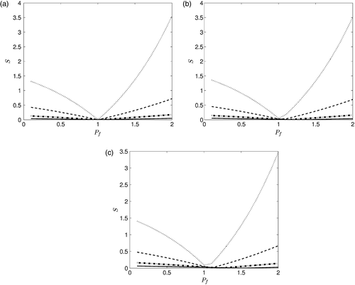
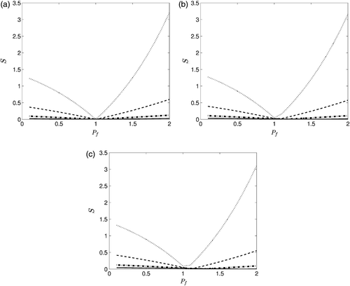
we determine its global minimum, which should be located at Pf = 1. illustrates the variation of S, as a function of Pf∈(0,2], when
, where
,
, denote the boundary element midpoint nodes of a uniform discretization of the time interval [0,tf = 1]. As one may notice in , the computation for the plot associated with
would have been facing ‘a corner effect’, thus it is affected by significant errors near the origin. However, we can remove this effect by solving the problem again, using the same number of boundary elements N, for a new final time tf ≔ (1/N), and in this way the time boundary element node
, from the initial computation, becomes the new
. In some sense, this is a mesh refinement near the origin. In doing so, the minimum is now correctly located at Pf ≈ 1 (). Because of the big difference in scales between the plots corresponding to
, which are of the order of 10−3, relative to the ones corresponding to
, which are of the order of 1 in , we recast the first two ones separately in . Overall, from it can be seen that the minimum of the curves is indeed located close to Pf ≈ 1, with the accuracy increasing as t0 increases. In addition, the minimum becomes sharper as t0 increases.
Figure 1. Variation of S with Pf when (a) the flux measurement is taken at without refinement, (b) the flux measurement is taken at
with refinement and (c) the flux measurement is taken at
with refinement. Note: In all cases we have: dotted line for to
, dashed line for
, dash-dot line for
, and solid line for
.
We consider now the inverse coefficient identification problem given by (90)–(93) for the case of the flux measurement (10) at the right boundary x = 1, namely
(102)
Using the transformation (64), the converted problem (96)–(99) receives the flux measurement
(103)
Using again the BEM for solving (96)–(99), we obtain (∂v/∂x)(1,t0;Pf). By plotting the function
(104)
we determine the global minimum, which should be located at Pf = 1. The corner effect is again avoided by using the technique described in the case of the flux measurement at x = 0.
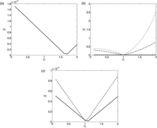
illustrates the variation of S, as a function of Pf ∈ (0, 2], when . Again, because of the difference in scale between the plots corresponding to
, which are of the order of 10−2, relative to the ones corresponding to
, which are of the order 1, we recast the former ones separately in . By comparing Figures and , we notice that the numerical results have a very similar structure for the two types of flux measurements at x = 0 and x = 1.
Figure 2. Variation of S with Pf when (a) the flux measurement is taken at and (b) the flux measurement is taken at
. Note: In both (a) and (b) we have: dotted line for
, dashed line for
, dash-dot line for
and solid line for
.
Another important aspect is the effect of perturbed data in the flux measurement (86), which allows us to investigate the stability of the numerical solution. Here we take
(105)
where, throughout the article, ρ is considered the percentage of perturbation (noise) up to 4%. Of course, since there is only one measurement, see Equations (9–12), all that is included in Equation (105) is in fact a ρ% perturbation of h1 from its exact value.
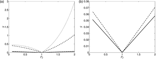
shows the variation of S given by (104), as a function of Pf ∈ (0, 2], when . From this figure it can be seen, as expected also from (88), that the stability of Pf decreases as t0 decreases. However, for a sufficiently large t0, such as
, the numerical results for Pf shown in are of comparable errors from the exact solution Pf = 1 as is the error 2ρe− t0 in the input measurement (105).
Figure 3. Variation of S with Pf when the flux measurement is taken at for cases: (a) ρ = 2% and (b) ρ = 4%. Note: In all cases we have: dotted line for
, dashed line for
, dash-dot line for
and solid line for
.
Next, we illustrate that the problem (90)–(93) maintains the same general behaviour when, as additional information, one employs either the internal temperature, (11) or the average temperature, (12), measurement.
Considering first the internal temperature measurement (11), namely
(106)
the change of variable (64) transforms (106) into the internal measurement
(107)
associated with the converted problem (96)–(99).
In order to illustrate typical numerical results, using the BEM for solving (96)–(99), we compute v(x0, t0; Pf), for internal temperatures taken at . We plot the function
, given by
(108)
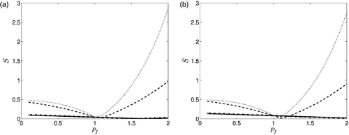
hoping to obtain a curve with the global minimum located closely to the point Pf = 1. illustrates the variation of S given by (108), as a function of Pf ∈ (0, 2], when x0 = 0.5,
perturbation is included in the measurements (106), as
(109)
From , it can be seen that the minimum of S is indeed achieved closely to Pf ≈ 1 – , showing also the good stability of the numerical results when the noisy data (109) are inverted – .
Figure 4. Variation of S with Pf when the temperature measurement data is taken at the interior points for: (a) exact data, i.e. ρ = 0, (b) ρ = 2%, and (c) ρ = 4%. Note: In all cases we have: dotted line for
, dashed line for
, dash-dot line for
and solid line for
.
The final numerical test that we have considered for the example (89) is for the case of the average temperature measurement (12), namely
(110)
In this case, the change of variable (64) transforms (110) into
(111)
By applying the BEM for solving (96)–(99), we obtain ∫0¹v(x,t0;Pf)dx and then plot the function
(112)
illustrates the variation of S given by (112), as a function of Pf ∈ (0, 2], when
perturbation is included in the measurements (110), as
(113)
The same conclusions as those drawn form are obtained.
6. Conclusions
This work initially develops an analytical framework for the inverse coefficient identification problem regarding the determination of the constant perfusion coefficient in the transient bio-heat conduction equation. The additional information provided either through a flux measurement, an internal temperature measurement or an average temperature measurement, is used to ensure the uniqueness of the inverse problem. Provided that any of these measurements belong to a certain theoretically argued interval, the solution of the inverse problem is also proved that it exists. Moreover, from the proofs we have carried out in both steady and unsteady cases, the existence of the unique solution associated to the inverse problem turned out to be equivalent to the fact that the corresponding perfusion coefficient is actually the unique positive solution of a non-linear algebraic equation. In the presence of homogeneous boundary conditions, we have given explicit, necessary and sufficient conditions for the existence and uniqueness of solution.
For arbitrary initial and boundary conditions, we used numerical techniques to compute the perfusion coefficient Pf. We used for this the BEM combined with an ordinary minimization on a test example that considers all the four types of additional information discussed. In all cases, the numerical results are accurate and stable with respect to noisy perturbations of the input data. Further, it was noticed that the stability of the solution increases with respect to increasing the non-dimensional time instant t0 at which the additional measurement is recorded. Other examples that are closer to reality will be attempted once the practical data are available from the medical laboratories.
In future work, we will extend the analysis performed in this article to the inverse problem of recovering a time-dependent perfusion coefficient.
Acknowledgements
The first author would like to acknowledge the European Union, European Research Commission, which fully supported the research work and attended this conference through the award of a Marie Curie Research Fellowship in the Centre for Computational Fluid Dynamics at The University of Leeds. The authors would also like to thank for the constructive comments made by the referees.
References
- Chato, JC, 1990. Fundamentals of Bioheat Transfer. Berlin: Springer-Verlag; 1990.
- Liu, J, and Xu, LS, 2000. Boundary information based diagnostic on the thermal states of biological bodies, Int. J. Heat Mass Transfer 43 (2000), pp. 2827–2839.
- Pennes, HH, 1948. Analysis of tissue and arterial blood temperature in the resting human forearm, J. Appl. Physiol. 1 (1948), pp. 93–122.
- Chan, CL, 1992. Boundary element method analysis for the bioheat transfer equation, J. Biomech. Eng.– Trans. ASME. 114 (1992), pp. 358–365.
- Ren, ZP, Liu, J, and Wang, CC, 1995. Boundary element method (BEM) for solving normal and inverse bio-heat transfer problem of biological bodies with complex shape, J. Therm. Sci. 4 (1995), pp. 117–124.
- Strohbehn, JW, and Roemer, RB, 1984. A survey of computer simulation of hypothermia treatments, IEEE Trans. Bio-Med. Eng. 31 (1984), pp. 136–149.
- Kleinman, AM, and Roemer, RB, 1983. A direct substitution, equation error technique for solving the thermographic tomography problem, J. Biomech. Eng.– Trans. ASME. 105 (1983), pp. 237–243.
- Hartman, P, and Wintner, A, 1950. On the solutions of the equations of heat conduction, Am. J. Math. 72 (1950), pp. 367–395.
- Stroock, DW, 1994. A Concise Introduction to the Theory of Integration. Boston: Birkhauser Boston, Inc.; 1994.
- Cannon, JR, 1964. Determination of certain parameters in heat conduction, J. Math. Anal. Appl. 8 (1964), pp. 188–201.
- Tikhonov, AN, and Samarskii, AA, 1963. Equations of Mathematical Physics. New York: Pergamon; 1963.
- Brebbia, CA, Telles, JCF, and Wrobel, LC, 1984. Boundary Element Techniques: Theory and Applications in Engineering. Berlin: Springer-Verlag; 1984.
- Lesnic, D, 2006. Post-Graduate Course on the Boundary Element Method. CCFD-5070. Centre for Computational Fluid Dynamics, University of Leeds; 2006.
